There is also more information on benchmarking, including how to reproduce the results, in the benches/ directory of the jsongrep repository.
原文
This article is both an introduction to a tool I have been working on called jsongrep, as well as a technical explanation of the internal search engine it uses. I also discuss the benchmarking strategy used to compare the performance of jsongrep against other JSON path-like query tools and implementations.
In this post I'll first show you the tool, then explain why it's fast (conceptually), then how it's fast (the automata theory), and finally prove it (benchmarks).
Upfront I would like to say that this article is heavily inspired by Andrew Gallant's amazing
ripgreptool, and his associated blog post "ripgrep is faster than {grep, ag, git grep, ucg, pt, sift}".
Table of Contents
You can install jsongrep from crates.io:
cargo install jsongrepLike ripgrep, jsongrep is cross-platform (binaries available here) and written in Rust.
jsongrep (jg binary) takes a query and a JSON input and prints every value whose path through the document matches the query. Let's build up the query language piece by piece using this sample document:
sample.json:
{
  "name": "Micah",
  "favorite_drinks": ["coffee", "Dr. Pepper", "Monster Energy"],
  "roommates": [
    {
      "name": "Alice",
      "favorite_food": "pizza"
    }
  ]
}
Dot paths select nested fields by name. Dots (.) between field names denote concatenation-- "match this field, then that field":
$ cat sample.json | jg 'roommates[0].name'
roommates.[0].name:
"Alice"
Wildcards match any single key (*) or any array index ([*]):
$ cat sample.json | jg 'favorite_drinks[*]'
favorite_drinks.[0]:
"coffee"
favorite_drinks.[1]:
"Dr. Pepper"
favorite_drinks.[2]:
"Monster Energy"
Alternation (|) matches either branch, like regex alternation:
$ cat sample.json | jg 'name | roommates'
name:
"Micah"
roommates:
[
  {
    "name": "Alice",
    "favorite_food": "pizza"
  }
]
Recursive descent uses * and [*] inside a Kleene star to walk arbitrarily deep into the tree. For example, to find every name field at any depth:
$ cat sample.json | jg '(* | [*])*.name'
name:
"Micah"
roommates.[0].name:
"Alice"
The pattern (* | [*])* means "follow any key or any index, zero or more times", e.g., descend through every possible path. The trailing .name then filters for only those paths that end at a field called name.
Equivalently, jg exposes the -F ("fixed string") flag as a shorthand for these recursive descent queries:
$ cat sample.json | jg -F name
name:
"Micah"
roommates.[0].name:
"Alice"
Optional (?) matches zero or one occurrence:
$ cat sample.json | jg 'roommates[0].favorite_food?'
roommates.[0]:
{
  "name": "Alice",
  "favorite_food": "pizza"
}
roommates.[0].favorite_food:
"pizza"
Notice how the inner string "pizza" matches with the ?, in addition to the parent zero-occurrence case.
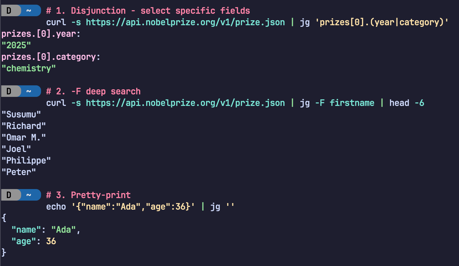
Here's a screenshot showing several of these features in action: Example of some of jsongrep's search query features in practice.
NOTE:
jsongrepis smart about detecting if you are piping to another command likelessorsort, in which case it will not display the JSON paths. This can be overridden though if desired with the--with-pathoption.
JSON documents are trees: objects and arrays branch, scalars are leaves, and keys and indices label the edges. Querying a JSON document is really about describing paths through this tree. jsongrep takes this observation literally: its query language is a regular language over the alphabet of keys and indices. Think regular expressions, but instead of matching characters in a string, you're matching edges in a tree.
Why does "regular" matter? Because regular languages have a well-known, powerful property: they can be compiled into a deterministic finite automaton (DFA). A DFA processes input in a single pass with $O(1)$ work per input symbol-- no backtracking, no recursion stack, no exponential blowup on pathological queries. The query is paid for once at compile time, then search is essentially free.
This is the key difference from tools like jq, jmespath, or jsonpath-rust. Those tools interpret path expressions: at each node in the JSON tree, they evaluate the query, check predicates, and recursively descend into matching branches. If a query involves recursive descent (.. or $..), these tools may revisit subtrees or maintain worklists. jsongrep does something fundamentally different-- it compiles the query into a DFA before it ever looks at the JSON, then walks the document tree exactly once, taking a single $O(1)$ state transition at each edge. No interpretation, no backtracking, one pass.
As a consequence, End-to-end search performance comparison over the xlarge (~190 MB) dataset.jsongrep is fast-- like really fast:
Again borrowing from the ripgrep blog post, here's an "anti-pitch" for jsongrep:
jsongrepis not as ubiquitous (yet) asjq.jqis the go-to for JSON querying, filtering, and transductions.The query language is deliberately less expressive than
jq's.jsongrepis a search tool, not a transformation tool-- it finds values but doesn't compute new ones. There are no filters, no arithmetic, no string interpolation.jsongrepis new and has not been battle-tested in the wild.
Keep reading if interested in the internals of
jsongrep!
With the tool overview and motivation out of the way, let's dive into the internals. This section traces a single query through every stage of the engine.
The Pipeline at a Glance
The core of the search engine is a five-stage pipeline:
- Parse the JSON document into a tree via
serde_json_borrow(zero-copy). - Parse the user's query into a
QueryAST. - Construct an NFA from the query via Glushkov's construction algorithm.
- Determinize the NFA into a DFA via subset construction
- Walk the JSON tree, taking DFA transitions at each edge and collecting matches.
To make this concrete, we'll trace the query roommates[*].name through every stage. Given our sample document, this query should match "Alice" at path roommates[0].name.
Parsing the Query
The query string roommates[*].name is parsed into an AST. jsongrep uses a PEG grammar (via the pest library) that maps the query DSL to a tree of Query enum variants:
Slightly cleaned-up pretty Debug of the compiled roommates[*].name Query:
Sequence(
    [
        Sequence(
            [
                Field("roommates"),
                ArrayWildcard,
            ],
        ),
        Field("name"),
    ],
)
The grammar is intentionally simple. Dots denote concatenation (sequencing), | denotes alternation (disjunction), postfix * denotes Kleene star (zero or more repetitions), and postfix ? denotes optional (zero or one). Parentheses group subexpressions. This maps directly to the definition of a regular language-- and that's the whole point. Because the query language is regular, everything that follows (NFA, DFA, single-pass search) is possible.
The full Query AST supports these variants:
| Variant | Syntax | Example |
|---|---|---|
Field | name or "quoted name" | roommates |
Index | [n] | [0] |
Range | [start:end] | [1:3] |
RangeFrom | [n:] | [2:] |
FieldWildcard | * | * |
ArrayWildcard | [*] | [*] |
Optional | e? | name? |
KleeneStar | e* | (* | [*])* |
Disjunction | a | b | name | age |
Sequence | a.b | foo.bar |
JSON as a Tree
JSON values form a tree. Object keys and array indices are the edges; the values they point to are the nodes. Scalars (strings, numbers, Booleans, null) are leaves.
Our sample document forms this tree: Sample JSON document as a tree.
A query, then, describes a set of paths from the root to matching nodes. The query roommates[*].name describes the path: take the roommates edge, then any array index, then the name edge.
Constructing the NFA (Glushkov's Algorithm)
With the query parsed into an AST, we need to convert it into an automaton that can match paths. The first step is building a nondeterministic finite automaton (NFA).
jsongrep uses Glushkov's construction, which has a key advantage over the more common Thompson's construction: it produces an $\epsilon$-free NFA. Every transition in the resulting NFA consumes a symbol-- no epsilon transitions to chase, which simplifies the downstream determinization.
Glushkov's algorithm works in four steps:
1. Linearize the query. Each symbol (field name, wildcard, index range) in the query gets a unique position number. Our query roommates[*].name has three symbols:
| Position | Symbol |
|---|---|
| 1 | Field("roommates") |
| 2 | ArrayWildcard (any index) |
| 3 | Field("name") |
2. Compute the First and Last sets. The First set contains positions that can appear at the start of a match; the Last set contains positions that can appear at the end. For a simple sequence, First = {first element} and Last = {last element}:
- $\textit{First} = \set{1}$ (
roommates) - $\textit{Last} = \set{3}$ (
name)
3. Compute the Follows set. For each position i, Follows(i) is the set of positions that can immediately follow i in a valid match. For a simple sequence, each position follows the one before it:
- $\textit{Follows}(1) = \set{2}$
- $\textit{Follows}(2) = \set{3}$
- $\textit{Follows}(3) = \emptyset$
For queries with Kleene star or alternation, the $\textit{Follows}$ sets become more interesting-- loops and branches appear naturally.
4. Assemble the NFA. The NFA has $n + 1$ states (one start state plus one per position). Transitions are wired up from the computed sets:
- From the start state $q_0$, add transitions to every position in the $First$ set
- For each position $i$ and each $j \in \textit{Follows}(i)$, add a transition from state $i$ to state $j$ on symbol $j$
- States corresponding to positions in the $\textit{Last}$ set are marked accepting
For our query, the resulting NFA is:
Constructed NFA for `roommates[*].name`:
NFA States: 4
Start State: 0
Accepting States: [3]
First set: ["[0] Field(roommates)"]
Last set: ["[2] Field(name)"]
Factors set:
	[0] Field(roommates) can be followed by:
		[1] Range(0, 18446744073709551615)
	[1] Range(0, 18446744073709551615) can be followed by:
		[2] Field(name)
	[2] Field(name) cannot be followed
Transitions:
	state 0:
		on [0] Field(roommates) -> [1]
	state 1:
		on [1] Range(0, 18446744073709551615) -> [2]
	state 2:
		on [2] Field(name) -> [3]
	state 3:
The
18446744073709551615value is the value ofusize::MAXon my machine (64 bit address space, equal to2^64 - 1), which is the maximum value of a 64-bit unsigned integer.
The NFA transition table:
| State | Field("roommates") | [*] | Field("name") | Accepting? |
|---|---|---|---|---|
| $q_0$ | $q_1$ | — | — | No |
| $q_1$ | — | $q_2$ | — | No |
| $q_2$ | — | — | $q_3$ | No |
| $q_3$ | — | — | — | Yes |
The NFA state diagram:
$$q_0 \xrightarrow{\texttt{roommates}} q_1 \xrightarrow{[\ast]} q_2 \xrightarrow{\texttt{name}} q_3$$
This is a simple chain for our simple query, but for queries with * or |, the NFA would have branching and looping edges. For example, (* | [*])*.name would produce a state with self-loops on both FieldWildcard and ArrayWildcard, capturing the "descend through anything" behavior.
Determinizing: NFA to DFA (Subset Construction)
An NFA can be in multiple states simultaneously-- on a given input, it may have several valid transitions. This is fine theoretically but bad for performance: simulating an NFA means tracking a set of active states at each step. A DFA, by contrast, is in exactly one state at all times, meaning each transition is an O(1) table lookup. Importantly, Rabin and Scott showed that every NFA can be turned into an equivalent DFA.
The standard algorithm for converting an NFA to a DFA is subset construction (also called the powerset construction). The idea is simple: each DFA state corresponds to a set of NFA states. The algorithm explores all reachable sets via breadth-first search:
- Start with the DFA state corresponding to $q_0$ (just the NFA start state).
- For each DFA state and each symbol in the alphabet, compute the set of NFA states reachable by taking that transition from any NFA state in the current set.
- If this resulting set is new, create a new DFA state for it.
- A DFA state is accepting if any of its constituent NFA states is accepting.
- Repeat until no new DFA states are discovered.
For our example query roommates[*].name, the NFA is already deterministic (a simple chain with no branching), so subset construction produces a DFA with the same shape:
Constructed DFA for query: `roommates[*].name`
DFA States: 4
Start State: 0
Accepting States: [3]
Alphabet (4 symbols):
	0: Other
	1: Field("roommates")
	2: Field("name")
	3: Range(0, 18446744073709551615)
Transitions:
	state 0:
		on [Other] -> (dead)
		on [Field("roommates")] -> 1
		on [Field("name")] -> (dead)
		on [Range(0, 18446744073709551615)] -> (dead)
	state 1:
		on [Other] -> (dead)
		on [Field("roommates")] -> (dead)
		on [Field("name")] -> (dead)
		on [Range(0, 18446744073709551615)] -> 2
	state 2:
		on [Other] -> (dead)
		on [Field("roommates")] -> (dead)
		on [Field("name")] -> 3
		on [Range(0, 18446744073709551615)] -> (dead)
	state 3:
		on [Other] -> (dead)
		on [Field("roommates")] -> (dead)
		on [Field("name")] -> (dead)
on [Range(0, 18446744073709551615)] -> (dead)| DFA State | NFA States | Accepting? |
|---|---|---|
| 0 | $\set{q_0}$ | No |
| 1 | $\set{q_1}$ | No |
| 2 | $\set{q_2}$ | No |
| 3 | $\set{q_3}$ | Yes |
The transition table:
| State | Field("roommates") | Field("name") | Range(0, MAX) | Other | Accepting? |
|---|---|---|---|---|---|
| 0 | 1 | No | |||
| 1 | 2 | No | |||
| 2 | 3 | No | |||
| 3 | Yes |
So the DFA's state diagram looks like this:
$$q_0 \xrightarrow{\texttt{roommates}} q_1 \xrightarrow{[\ast]} q_2 \xrightarrow{\texttt{name}} q_3$$
In the implementation, the alphabet isn't just the literal symbols from the query-- jsongrep also adds an Other symbol to handle JSON keys that don't appear in the query. Any transition on Other leads to a dead state (or stays in a state where that key is irrelevant), ensuring we skip non-matching branches efficiently.
For more complex queries, subset construction can produce DFA states that combine multiple NFA states. For instance, (* | [*])*.name would produce DFA states representing sets like $\set{q_0, q_1}$ (both "at start" and "in the middle of descending"), which is what enables the single-pass behavior.
Searching: DFS with DFA Transitions
This is the payoff. With the DFA built, searching the JSON document is a simple depth-first traversal of the tree, carrying the DFA state along:
- Start at the root of the JSON tree in DFA state $q_0$.
- At each node, iterate over its children (object keys or array indices).
- For each child edge, look up the DFA transition: given the current state and the edge label (key name or index), what's the next state?
- If no transition exists for this edge, skip the subtree entirely.
- If the new state is accepting, record the match (path + value).
- Recurse into the child with the new DFA state.
Let's trace our query roommates[*].name against the sample document:
1. Start at the root object in DFA state $q_0$. Iterate over its three keys:
- Edge
"name": $\delta(q_0, \texttt{Field("name")}) \to \text{dead}$. Prune this subtree. - Edge
"favorite_drinks": $\delta(q_0, \texttt{Other}) \to \text{dead}$. Prune. - Edge
"roommates": $\delta(q_0, \texttt{Field("roommates")}) \to q_1$. Descend.
2. At the roommates array in state $q_1$. Iterate over its indices:
- Edge
[0]: $\delta(q_1, \texttt{Range(0, MAX)}) \to q_2$. Descend.
3. At the roommates[0] object in state $q_2$. Iterate over its keys:
- Edge
"name": $\delta(q_2, \texttt{Field("name")}) \to q_3$. State $q_3$ is accepting-- record the match:roommates.[0].name→"Alice". - Edge
"favorite_food": $\delta(q_2, \texttt{Other}) \to \text{dead}$. Prune.
4. Search complete. One match found:
roommates.[0].name:
"Alice"
Notice how the DFA let us skip the "name" and "favorite_drinks" subtrees at the root in step 1-- we never even looked at their values. On a large document, this pruning is what makes the search fast: entire branches of the JSON tree are discarded in $O(1)$ without recursing into them.
Every node is visited at most once, and each transition is an $O(1)$ table lookup. The total search time is O(n) where n is the number of nodes in the JSON tree. No backtracking, no interpretation overhead.
As an implementation bonus, jsongrep uses serde_json_borrow for zero-copy JSON parsing. The parsed tree holds borrowed references (&str) into the original input buffer rather than allocating new strings, which significantly reduces memory overhead on large documents.
All benchmarks use Criterion.rs, a statistics-driven Rust benchmarking framework that provides confidence intervals, outlier detection, and change detection across runs.
Datasets
Four datasets of increasing size test scaling behavior:
Compared Tools
Five JSON query tools were compared:
Benchmark Groups
The benchmarks are split into four groups to isolate where time is spent:
document_parse-- JSON parsing cost only. Measuresserde_json_borrow(zero-copy) vs.serde_json::Value(allocating) vs.jmespath::Variable. This isolates jsongrep's zero-copy parsing advantage.query_compile-- Query compilation cost only. jsongrep must build an AST and construct a DFA upfront; other tools may have cheaper (or no) compile steps. This is the price jsongrep pays for fast search.query_search-- Pre-compiled query, pre-parsed document, search only. Isolates the traversal/matching cost without parse or compile overhead.end_to_end-- The full pipeline: parse JSON + compile query + search. This is the realistic CLI usage scenario.
Equivalent Queries
Each tool uses its own query syntax, but the benchmarks ensure equivalent work across tools. For example:
| Concept | jsongrep | JSONPath | jq |
|---|---|---|---|
| Simple field | name | $.name | .name |
| Nested path | name.first | $.name.first | .name.first |
| Array index | hobbies[0] | $.hobbies[0] | .hobbies[0] |
| Recursive descent | (* | [*])*.description | $..description | .. | .description? // empty |
Fairness Considerations
- The zero-copy parsing advantage is explicitly isolated in the
document_parsegroup, not hidden. jsongrep's upfront DFA compilation cost is measured separately inquery_compile, so readers can see the tradeoff.- Tools lacking certain query features (e.g.,
jmespathhas no recursive descent) are skipped for those benchmarks rather than penalized. - Tools requiring ownership of parsed JSON (
jaq,jmespath) use Criterion'siter_batchedto fairly separate cloning costs from search costs.
Let's take a look at the results from the benchmarks. We'll use the xlarge dataset unless otherwise noted since it provides the best demonstration of performance impacts, but the full results are available here.
Document Parse Time

Document parse times on xlarge dataset across all tools.
No surprises here: serde_json_borrow is the fastest, followed by serde_json::Value and jmespath::Variable.
Query Compile Time
As expected, jsongrep query compile time.jsongrep takes time to compile the different queries and this is its largest cost:
Compare this to the compile time of jmespath query compile time.jmespath (an order of magnitude faster):
Search Time

Searches times on xlarge dataset across all tools.
All query_search xlarge results
End-to-End Search Time
As shown at the beginning of the post, over the xlarge (~190 MB) dataset on the end-to-end benchmark, it's not even close: End-to-end search performance comparison over the xlarge (~190 MB) dataset.
The full, interactive Criterion report is available at the live benchmarking site.
jsongrep is entirely open-source, MIT-licensed software.
jsongrep also exposes its DFA-based query engine as a library crate, so you can embed fast JSON search directly in your own Rust projects.