I’ve been working on improving how we schedule maintenance in Akamai’s cloud infrastructure, especially disruptive maintenance on hypervisor hosts serving hundreds of thousands of guest VMs. The problem is fairly complex, with competing constraints such as capacity, customer disruption SLAs, and concurrency limits across hosts, racks, and datacenters.
While prototyping solutions, I tried several optimization tools, including commercial and open-source MIP solvers. After exploring different options, I found Google’s OR-Tools library, particularly its CP-SAT solver, to be a strong fit for scheduling problems. In this post, I’ll walk through a simple scheduling model in OR-Tools and explain why it works well for this kind of problem.
Maintenance Scheduling in Cloud Infrastructure
First, let me explain the problem I’m trying to solve. Cloud providers manage physical servers called “hypervisor hosts” that run virtual machines (VMs) for customers. These hosts need periodic maintenance to ensure security and reliability. Some of these maintenance tasks can be done with live patches that don’t require a reboot. Handling live patches is relatively straightforward, and the main challenge is safely rolling out updates. However, some maintenance tasks require a reboot of the host. Before the host is rebooted, all VMs on it need to be migrated to other hosts. This process is disruptive to customers, so it requires careful scheduling to minimize the impact while still making sure all maintenance tasks are completed in a reasonable time frame.
The process of evacuating multiple hosts for maintenance involves a complex scheduling problem with several constraints. The main challenges can be summarized as the “3Cs”:
Capacity: Evacuating hosts requires spare capacity in the datacenter to accommodate the migrated VMs.
Concurrency: Migrations are resource-intensive operations. They use CPU, disk I/O, and network bandwidth. Only a limited number of migrations can be performed concurrently without overloading the hosts or the network.
Conflict: Customers tolerate a certain amount of disruption during maintenance, but planned maintenance should not cause too much disruption. This means only a small portion of any given customer’s VMs can be migrated at the same time.
With these challenges in mind, the goal of the scheduling problem is to find a schedule for the maintenance tasks that minimizes the total time to complete all maintenance while respecting these constraints.
If you’re interested in this problem, feel free to check out my SRECon26 presentation: Keeping a Hypervisor Fleet Up to Date with Minimal Customer Disruption
How to Model the Problem
Operations Research (OR) is a well-established field that uses algorithms and mathematical models to solve complex decision-making problems. OR researchers have been working on scheduling problems for decades, and they have come up with various “problem types” that capture the essence of different scheduling challenges. Some well-known problem types include Job Shop Scheduling, Flow Shop Scheduling, and Resource-Constrained Project Scheduling. Knowing the right problem type for your scheduling problem helps you leverage the existing research and algorithms that have already been developed for it.
Maintenance scheduling in the cloud is close to a Resource-Constrained Project Scheduling Problem (RCPSP) without the precedence constraints. In RCPSP, you have a set of tasks that need to be scheduled, each with its own duration and resource requirements. The goal is to find a schedule that minimizes the overall project duration while respecting resource constraints. Similarly, in maintenance scheduling, each VM migration can be seen as a task that requires certain resources (see the 3Cs above), and the goal is to minimize the total time needed to complete all maintenance tasks.
OR-Tools is an open-source software suite developed by Google that provides a collection of tools for solving combinatorial optimization problems. One of its key components is the CP-SAT solver, which is a versatile portfolio solver that can handle a wide range of scheduling problems. For any given problem, CP-SAT tries a range of algorithms and shares information between them.
CP-SAT is particularly well-suited for scheduling problems because it has specialized variables and constraints for modeling time, which makes modeling scheduling problems more intuitive and efficient.
Let me give you code examples to illustrate this point. First, let’s set up a toy problem for ourselves, where we have a single hypervisor host that needs to be maintained, and we have 3 VMs that need to be migrated off of it. Let’s assume each migration takes 10 time units, and we want to consider solutions that can be completed within 100 time units.
hosts = ["host_1"]
vms = {"host_1": ["vm_1", "vm_2", "vm_3"]}
migration_duration = 10
planning_horizon = 100
The core of the problem is to schedule the migrations of these VMs while respecting the constraints related to capacity, concurrency, and conflict. So we need to model the timing of these migrations and the resources they consume. This is where CP-SAT’s interval variables come in handy. In CP-SAT, you can use interval variables to represent tasks that have a start time, end time, and duration. Let’s create an interval variable for each VM migration and save them in a dictionary for easy access later on.
vm_interval_vars = {} # Dictionary to hold interval variables for each VM

for host in hosts:
    vm_interval_vars[host] = {}
    for vm in vms[host]:
        start_var = model.new_int_var(0, planning_horizon, f"{vm}_start")
        end_var = model.new_int_var(0, planning_horizon, f"{vm}_end")
        migration_duration = 10

        vm_interval_var = model.new_interval_var(
            start=start_var, size=migration_duration, end=end_var, name=f"{vm}_interval"
        )

        vm_interval_vars[host][vm] = vm_interval_var
Executing the above code will give you a dictionary vm_interval_vars that contains interval variables for each VM’s migration. Each interval variable has a start time, end time, and a fixed duration of 10 time units.
{
    'host_1': {
        'vm_1': vm_1_interval(start = vm_1_start, size = 10, end = vm_1_end),
        'vm_2': vm_2_interval(start = vm_2_start, size = 10, end = vm_2_end),
        'vm_3': vm_3_interval(start = vm_3_start, size = 10, end = vm_3_end)
    }
}
Interval variables make it easy to express constraints related to concurrency and resource usage. For example, you can use the AddNoOverlap constraint to ensure that no two migrations that require the same resource, such as network bandwidth, overlap in time.
for host, vms_dict in vm_interval_vars.items():
    vm_intervals = list(vms_dict.values())
    model.AddNoOverlap(vm_intervals)
Or better, you can use the AddCumulative constraint to model limited resource capacity and ensure that total resource usage at any given time does not exceed the available capacity. The constraint below sets a limit on the number of concurrent migrations that can happen at the same time. To match the AddNoOverlap constraint above, we can set the maximum number of concurrent migrations to 1:
maximum_migrations_per_host = 1

for host, vms_dict in vm_interval_vars.items():
    vm_intervals = list(vms_dict.values())

    model.AddCumulative(
        vm_intervals,               # List of interval variables
        [1] * len(vm_intervals),    # Resource usage for each interval variable
        maximum_migrations_per_host # Maximum resource capacity
    )
The second argument in AddCumulative is the list of resource usages for each interval variable, which in this case is simply 1 for each migration since each migration consumes one unit of the resource. A more powerful use of AddCumulative is to assign different resource usages to different migrations, which is more useful for modeling real constraints such as throughput. If some VMs can be migrated with higher throughput than others, instead of limiting the number of concurrent migrations, you can limit total throughput at any given time:
migration_throughput = {"vm_1": 5, "vm_2": 3, "vm_3": 2}
host_maximum_throughput = 5

for host, vms_dict in vm_interval_vars.items():
    vm_intervals = list(vms_dict.values())
    vm_throughputs = [migration_throughput[vm] for vm in vms_dict.keys()]

    model.AddCumulative(vm_intervals, vm_throughputs, host_maximum_throughput)
Since the maximum throughput is 5, we would expect the schedule to migrate VMs 2 and 3 at the same time, but not VM 1 with any other VM, because VM 1 alone consumes all available throughput.
At this point, we have a tiny model that captures one aspect of the maintenance scheduling problem, which is the concurrency constraint. Let’s solve this model and see what the solution looks like:
solver = cp_model.CpSolver()
status = solver.Solve(model)
print(status)
# Print the schedule
if status == cp_model.OPTIMAL or status == cp_model.FEASIBLE:
    for host, vms_dict in vm_interval_vars.items():
        print(f"Schedule for {host}:")
        for vm, interval_var in vms_dict.items():
            start = solver.Value(interval_var.StartExpr())
            end = solver.Value(interval_var.EndExpr())
            print(f"  {vm}: Start at {start}, end at {end}")
else:
    print("No solution found.")
The solution prints the start and end times for each VM migration, which gives you a schedule that respects the concurrency constraint.
CpSolverStatus.OPTIMAL
Schedule for host_1:
  vm_1: Start at 10, end at 20
  vm_2: Start at 0, end at 10
  vm_3: Start at 0, end at 10
As expected, we see VM 2 and VM 3 being migrated at the same time, while VM 1 is migrated separately to respect the maximum throughput constraint.
To understand why OR-Tools is a great choice, it helps to understand the alternatives. Another common technique for solving scheduling problems is Mixed Integer Programming (MIP). There are many open-source MIP solvers out there, but none of them give you tools to model time and scheduling constraints as naturally.
There are two ways to solve this scheduling problem with MIP: a time-indexed formulation and a time-continuous formulation. The time-indexed formulation is intuitive, but it does not scale well as the number of tasks and the planning horizon increase. The time-continuous formulation is more efficient, but it is less intuitive and requires a lot of effort to get right.
“Easy” MIP Method: Time-Indexed Formulation
The easy way to implement a scheduling problem with MIP is to use a time-indexed formulation, where you create binary variables that indicate whether a task is active at a specific time. For example, you can create a binary variable active[i, t] that is 1 if task i is active at time t, and 0 otherwise. Then, you can add constraints to ensure that the total resource usage at any given time does not exceed the available capacity.
To demonstrate a small example, I will use Pyomo to model the same problem as above with a time-indexed formulation.
First, let’s define the sets and variables. Similar to above, we need a variable for each VM’s start time. In addition, we also need a binary variable to indicate whether the VM is actively migrating at time t.
model = pyo.ConcreteModel()

# Sets
model.VMS = pyo.Set(initialize=vms["host_1"])
model.TIME = pyo.RangeSet(0, planning_horizon)

# Variables
# Start time for each VM migration
model.start = pyo.Var(
    model.VMS, domain=pyo.NonNegativeIntegers, bounds=(0, planning_horizon)
)
# Binary variable: is VM migrating at time t?
model.vm_active = pyo.Var(model.VMS, model.TIME, domain=pyo.Binary)

# Objective: Minimize makespan (completion time of last migration)
model.makespan = pyo.Var(domain=pyo.NonNegativeReals, bounds=(0, planning_horizon))
model.obj = pyo.Objective(expr=model.makespan, sense=pyo.minimize)
However, this approach can lead to a very large number of variables and constraints, especially if the planning horizon is long or if there are many tasks. This can make the model difficult to solve and may not scale well.
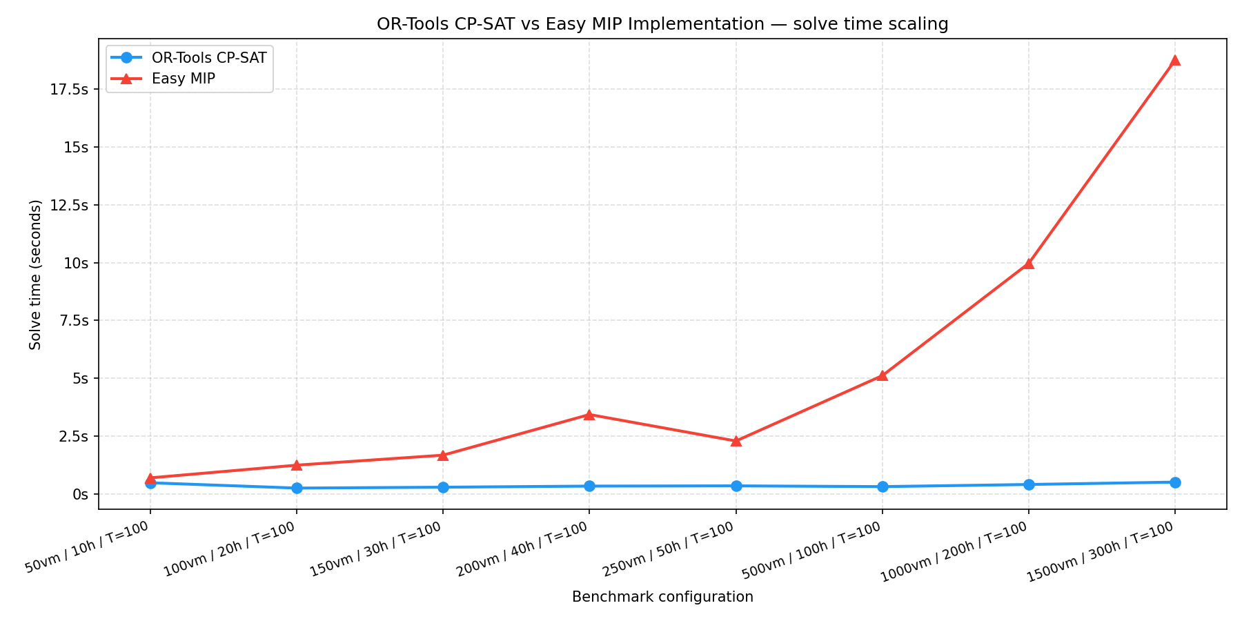
The graph below shows how the solve time of the time-indexed formulation grows as we increase the number of VMs and the planning horizon. As you can see, the solve time grows exponentially, which makes it impractical for larger problems.

Time-Continuous Formulation for MIP
An alternative way to formulate the same problem is the time-continuous formulation. Instead of tracking whether a task is active at each discrete time step, you can drop the time index completely and introduce binary ordering variables between pairs of tasks. This is not an easy formulation to come up with, and it is not as intuitive as the CP-SAT formulation, but it can be more efficient for small problems with large planning horizons.
The core idea is this: for any two tasks i and j that share a resource, exactly one of them must come first. We encode this with a binary variable y[i, j] that equals 1 if task i finishes before task j starts.
model = pyo.ConcreteModel()

M = planning_horizon  # Big-M constant

model.VMS = pyo.Set(initialize=vms["host_1"])
model.VM_PAIRS = pyo.Set(initialize=[
    (i, j) for i in vms["host_1"] for j in vms["host_1"] if i != j
])

# Start time for each VM migration
model.start = pyo.Var(model.VMS, domain=pyo.NonNegativeIntegers, bounds=(0, planning_horizon))

# Ordering variable: y[i,j] = 1 means task i finishes before task j starts
model.y = pyo.Var(model.VM_PAIRS, domain=pyo.Binary)

# Makespan
model.makespan = pyo.Var(domain=pyo.NonNegativeReals, bounds=(0, planning_horizon))
model.obj = pyo.Objective(expr=model.makespan, sense=pyo.minimize)
For the no-overlap constraint (equivalent to AddNoOverlap in CP-SAT), we need two things: a constraint that enforces ordering when y[i,j] = 1, and a constraint that ensures exactly one ordering is chosen between each pair:
# If i precedes j (y[i,j]=1), then j must start after i ends
model.precedence = pyo.Constraint(
    model.VM_PAIRS,
    rule=lambda model, i, j: model.start[j] >= model.start[i] + migration_duration - M * (1 - model.y[i, j])
)

# exactly one ordering must hold
model.one_ordering = pyo.Constraint(
    model.VM_PAIRS,
    rule=lambda model, i, j: model.y[i, j] + model.y[j, i] == 1
)

# Makespan must be >= all end times
model.makespan_constraint = pyo.Constraint(
    model.VMS,
    rule=lambda model, i: model.makespan >= model.start[i] + migration_duration
)
The number of variables is now O(n²) in the number of VMs. If the problem has a small number of VMs and a long planning horizon, this may be a significant improvement over the O(n × T) of the time-indexed formulation. For a planning horizon of, say, 1440 minutes (one day), the time-indexed model creates 1440x more variables per task, which quickly overwhelms the solver.
However, in order to implement the AddCumulative constraint in CP-SAT, we need a much more complicated constraint. The challenge is that at the start time of each task i, you need to ensure the total throughput of all concurrent tasks does not exceed the host’s limit.
“Task j is active when task i starts” is itself a compound condition (start[j] <= start[i] and start[i] < start[j] + duration[j]), and linearizing it requires yet another binary variable per pair plus two more Big-M constraints per pair. This quickly becomes unwieldy and difficult to understand. I wasn’t able to find a good way to express this constraint efficiently in MIP, which is one of the reasons I prefer CP-SAT for this kind of problem.
Conclusion
It is important to choose the right tool for the job. Scheduling problems have a unique set of constraints that make them difficult to model and solve with MIPs. The OR-Tools CP-SAT provides powerful abstractions that let you model scheduling problems in an intuitive and efficient way. With CP-SAT’s AddNoOverlap and AddCumulative constraints, which make use of interval variables, it is much easier to express the concurrency and resource constraints that are common in scheduling problems. Writing the same model with MIP is possible, but it requires a lot of effort and expertise to get the formulation right. Even then, the resulting model may not perform as well as the CP-SAT formulation, especially as the problem size grows.
If you’re facing a scheduling problem, I’d strongly recommend trying OR-Tools CP-SAT.