This article is all about movement. Of a vehicle, or a robot, or something like a 3D printer.
A 3D printer is really just a specialized robot with a hot glue gun which it can move in multiple directions while squirting out molten plastic.
Position, Velocity, Acceleration …
Our robot, or print head, has a position in space and also a velocity which is how fast it is moving and an acceleration which is how rapidly that velocity is changing.
Velocity is just the derivative of position: how fast is our position changing. Acceleration is the derivative of velocity: how rapidly our velocity is increasing or decreasing.
These are all vectors in that they have both magnitude and direction but for (many) 3D printers and machines each axis is a separate mechanism, so this article is for now going to talk about them as if they were scalars, eg: just a positive or negative number.
… Jerk?
Jerk is the derivative of acceleration, which might seem like a pretty abstract thing to be worried about.
But imagine a mass in a box under constant acceleration. Springs inside the box are pushing the mass to cause it to accelerate too. But if we change the size or direction of the acceleration, the mass is going to slide around until it reaches a new equilibrium.
Now imagine the box is your skull and the mass is your brain. Jerk is real!
Higher Orders
There’s also higher derivatives which are sometimes called Snap, Crackle and Pop.
Snap (sometimes called Jounce) is the rate of change of Jerk; Crackle is the rate of change of Snap, etc. I don’t have as neat an illustration of what these physically mean but there seems to be a consensus that they, and presumably even higher derivatives, have an effect on vibration and so on of mechanisms, and so they should be minimized too.
Discontinuities
Our 3D printer or similar machine follows a path made up of many segments. Some segments have fixed position and velocity: while the printer is extruding or the CNC mill is cutting, it goes in a set direction at a set speed.
Other parts of the movement are more free: the printer just has to get to the right place for the start of its next fixed segment, as rapidly as is practical.
The problem is smoothly transitioning between segments. A discontinuity in velocity requires a large acceleration. A discontinuity in acceleration requires a large jerk. And so on. When we combine segments into a path, it is important to match the ends to prevent these discontinuities. So our apparently “free” transport segments are actually critical to support smooth transitions in and out of our “working” segments.
Transitions & Trajectories
So let’s look at a way to make our transitions smooth.
What we’re looking for is some kind of
Sigmoid Function
which has the right general shape.
The most obvious sigmoid functions is the Logistic Function which does indeed transition smoothly between 0 and 1 and has well defined derivatives, but unfortunately it only converges towards 0 and 1 whereas we want to get our transition over and done with in finite time.
There are other suitable functions though, including polynomials.
SmoothStep …
SmoothStep is a family of polynomial functions which smoothly transition across the range [0,1] in the domain [0,1] in a Sigmoid shape.
$ S_1(t) = \begin{cases}0, & if\ t \leq 0 \\ 3t^2 - 2t^3, & if\ 0 \leq t \leq 1 \\ 1, & if\ 1 \leq t\end{cases} $
Smoothstep is a polynomial function and so the first derivative $ S^\prime_1 $, is polynomial too:
$ S'_1(t) = \begin{cases}0, & if\ t \leq 0 \\ -6t^2 + 6t, & if\ 0 \leq t \leq 1 \\ 0, & if\ 1 \leq t\end{cases} $
and has the handy property that it is neatly zero at both ends. However, $ S''_1 $ does not have
this property. Our velocity at each end of our movement is zero, but our acceleration is not.
… and SmootherStep …
If we want acceleration to be zero at the beginning and end of our trajectory, we can use Smootherstep, which is a fifth-order polynomial with this property:
$ S_2(t) = \begin{cases}0, & if\ t \leq 0 \\ 6t^5 - 15t^4 +10t^3, & 0 \leq t \leq 1 \\ 1, & 1 \leq t\end{cases} $
$ S'_2(t) = \begin{cases}0, & if\ t \leq 0 \\ 30t^4 - 60t^3 + 30t^2, & 0 \leq t \leq 1 \\ 0, & 1 \leq t\end{cases} $
$ S''_2(t) = \begin{cases}0, & if\ t \leq 0 \\ 120t^3 - 180t^2 + 60t, & 0 \leq t \leq 1 \\ 0, & 1 \leq t\end{cases} $
… and SmoothnStep
The SmoothStep function can be worked out to an arbitrary depth, for example $ S_6 $ is a 13th-order polynomial:
$ S_6(t) = \begin{cases}0, & t \leq 0 \\ 924t^{13} - 6006t^{12} + 16380t^{11} - 24024t^{10} + 20020t^9 - 9009t^8 + 1716t^7, & 0 \leq t \leq 1 \\ 1, & 1 \leq t\end{cases} $
For the $ n $-th Smoothstep function, all derivatives up to the $ n $-th derivative start and end at zero:
$ S^{(m)}_n(0) = S^{(m)}_n(1) = 0 \qquad where \qquad 1 \leq m \leq n $
The next few examples all use Smootherstep $ S_2 $ because it is slightly less cumbersome
but we’ll come back to $ S_6 $ later.
Logistic Function
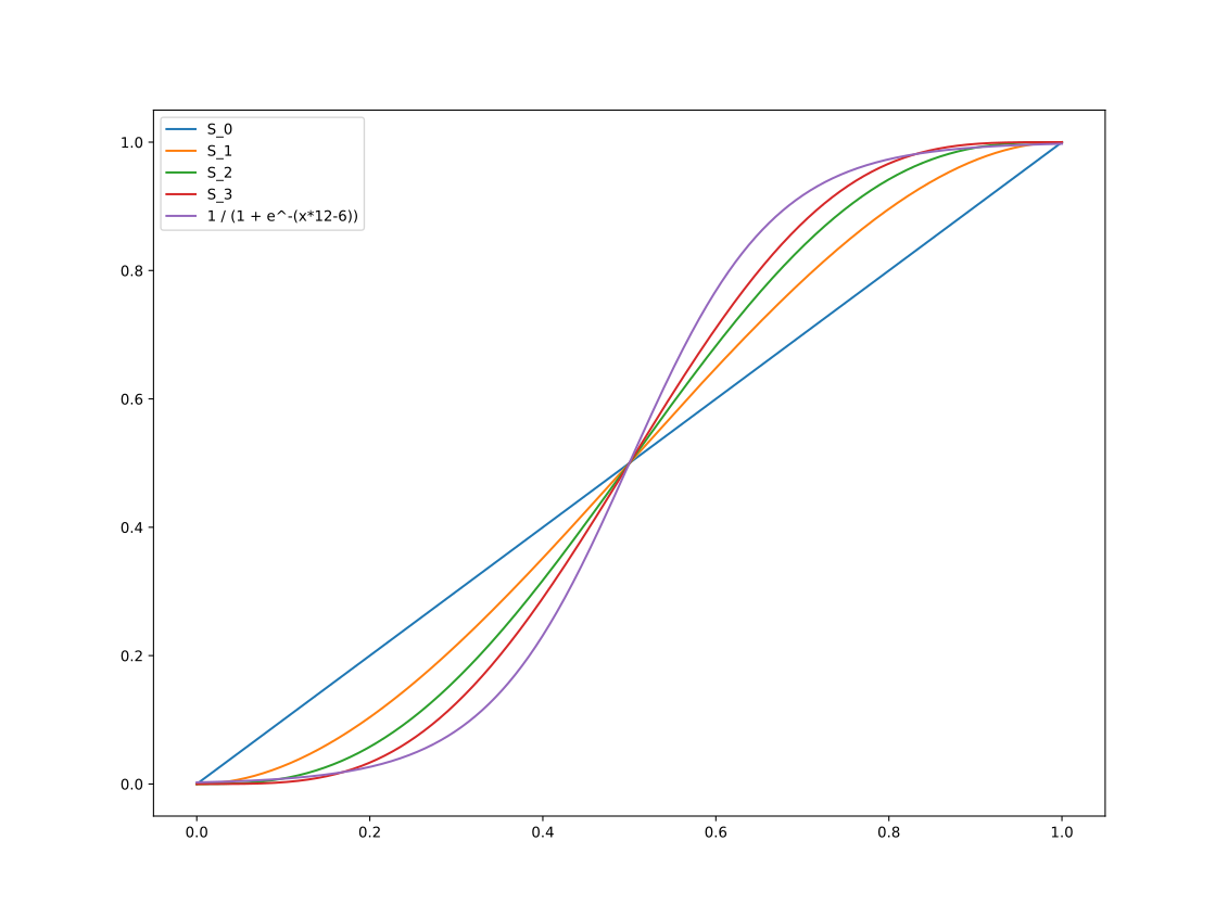
The higher the order of smoothstep, the more it resembles the Logistic Function except the tapered ends finish exactly at 0 and 1 instead of tapering off into infinity, which is handy for those of us who would like to actually finish moving.
This graph compares the first few Smoothstep functions with a scaled version
of the logistic function $ \frac{1}{1 + e^{6-12x}} $:

Some Python
If you want to mess around with these equations in Python, the numpy.polynomial library is rather handy.
Polynomial objects can be constructed from coefficients, and differentiated using the deriv method:
>>> from numpy.polynomial import Polynomial
>>> S_6 = Polynomial([0,0,0,0,0,0,0,1716,-9009,20020,-24024,16380,-6006,924], symbol='t')
>>> print(S_6)
0.0 + 0.0·t + 0.0·t² + 0.0·t³ + 0.0·t⁴ + 0.0·t⁵ + 0.0·t⁶ + 1716.0·t⁷ -
9009.0·t⁸ + 20020.0·t⁹ - 24024.0·t¹⁰ + 16380.0·t¹¹ - 6006.0·t¹² + 924.0·t¹³
>>> jerk = S_6.deriv(3)
>>> print(jerk)
0.0 + 0.0·t + 0.0·t² + 0.0·t³ + 360360.0·t⁴ - 3027024.0·t⁵ +
10090080.0·t⁶ - 17297280.0·t⁷ + 16216200.0·t⁸ - 7927920.0·t⁹ +
1585584.0·t¹⁰
>>> jerk(0)
np.float64(0.0)
>>> jerk(1)
np.float64(0.0)
From Here To There
So let’s work out a trajectory using SmootherStep.
Calculating $ S_2 $ is explained pretty well in wikipedia
but note that I’m using $ t $ as the free variable here since we’re using $ x $ for position and $ x(t) $ for position
varying with time.
First, we set up a 5th order polynomial with variable coefficients $ a_0, a_1, a_2, a_3, a_4, a_5 $
and consider its first and second derivatives:
$ S_2(t) = a_5 t^5 + a_4 t^4 + a_3 t^3 + a_2 x^2 + a_1 x + a_0 $
$ S'_2(t) = 5 a_5 t^4 + 4 a_4 t^3 + 3 a_3 t^2 + 2 a_2 t + a_1 $
$ S''_2(t) = 20 a_5 t^3 + 12 a_4 t^2 + 6 a_3 t + 2 a_2 $
We also know some values we expect to see for $ S_2 $ etc:
- Start from position 0, end up in position 1:
$ S_2(0) = 0 ; S_2(1) = 1 $ - Start and end with zero velocity:
$ S'_2(0) = 0 ; S'_2(1) = 0 $ - Start and end with zero acceleration:
$ S''_2(0) = 0 ; S''_2(1) = 0 $
So now we can use some Linear Algebra
to work out the coefficients $ a_n $ for our desired starting and finishing
values of $ S_2 $, $ S'_2 $ and $ S''_2 $.
$ \begin{bmatrix}0 & 0 & 0 & 0 & 0 & 1 \\ 1 & 1 & 1 & 1 & 1 & 1 \\ 0 & 0 & 0 & 0 & 1 & 0 \\ 5 & 4 & 3 & 2 & 1 & 0 \\ 0 & 0 & 0 & 2 & 0 & 0 \\ 20 & 12 & 6 & 2 & 0 & 0 \end{bmatrix} \begin{bmatrix} a_5 \\ a_4 \\ a_3 \\ a_2 \\ a_1 \\ a_0 \end{bmatrix} = \begin{bmatrix} S_2(0) \\ S_2(1) \\ S'_2(0) \\ S'_2(1) \\ S''_2(0) \\ S''_2(1) \end{bmatrix} = \begin{bmatrix} 0 \\ 1 \\ 0 \\ 0 \\ 0 \\ 0 \end{bmatrix} $
Solving this, we find:
$ \begin{bmatrix}a_5 \\ a_4 \\ a_3 \\ a_2 \\ a_1 \\ a_0 \end{bmatrix} = \begin{bmatrix}6 \\ -15 \\ 10 \\ 0 \\ 0 \\ 0 \end{bmatrix} $
So our polynomial is:
$ S_2(t) = 6 t^5 - 15 t^4 + 10 t^3 $
as expected.
This function makes a smooth transition from standing still at point 0 ($ x(0) = 0 ; x'(0) = 0 ; x''(0) = 0 $) to
standing still at point 1 ($ x(1) = 1 ; x'(1) = 0 ; x''(1) = 0 $)
Moving Targets
Our ‘target’ matrix can represent other situations of starting and finishing position, velocity and acceleration. For example we might be moving already from a previous trajectory, or we might want to be moving at the end of this trajectory, for example if it leads into a working trajectory.
For example here’s the same calculation but when our trajectory starts we’re already at point 1 and moving right:
$ x(0) = 1 \qquad ; \qquad x'(0) = 1 \qquad ; \qquad x''(0) = 0 $
… and when we end we’d like to be at point 2 and moving left:
$ x(1) = 2 \qquad ; \qquad x'(1) = -1 \qquad ; \qquad x''(1) = 0 $
(we’ll consider when we’d want to have $ x''(0) \neq 0 $ and/or $ x''(1) \neq 0 $ later)
$ \begin{bmatrix}0 & 0 & 0 & 0 & 0 & 1 \\ 1 & 1 & 1 & 1 & 1 & 1 \\ 0 & 0 & 0 & 0 & 1 & 0 \\ 5 & 4 & 3 & 2 & 1 & 0 \\ 0 & 0 & 0 & 2 & 0 & 0 \\ 20 & 12 & 6 & 2 & 0 & 0 \end{bmatrix} \begin{bmatrix} a_5 \\ a_4 \\ a_3 \\ a_2 \\ a_1 \\ a_0 \end{bmatrix} = \begin{bmatrix} x_0 \\ x_1 \\ x'_0 \\ x'_1 \\ x''_0 \\ x''_1 \end{bmatrix} = \begin{bmatrix} 1 \\ 2 \\ 1 \\ -1 \\ 0 \\ 0 \end{bmatrix} $
and solving we find:
$ \begin{bmatrix}a_5 \\ a_4 \\ a_3 \\ a_2 \\ a_1 \\ a_0 \end{bmatrix} = \begin{bmatrix}6 \\ -14 \\ 8 \\ 0 \\ 1 \\ 1 \end{bmatrix} $
More Python
We can use numpy’s linear algebra solver to find a solution for our situation and use this to produce a Polynomial
just for this segment of our trajectory:
>>> import numpy
>>> A = [[0,0,0,0,0,1],[1,1,1,1,1,1],[0,0,0,0,1,0],[5,4,3,2,1,0],[0,0,0,2,0,0],[20,12,6,2,0,0]]
>>> T1 = [0,1,0,0,0,0]
>>> M1 = numpy.linalg.solve(A,T1)
>>> print(M1)
[  6. -15.  10.   0.   0.   0.]
>>> T2 = [1,2,1,-1,0,0]
>>> M2 = numpy.linalg.solve(A,T2)
>>> print(M2)
[  6. -14.   8.   0.   1.   1.]
>>> p = numpy.polynomial.Polynomial(M2[::-1], symbol='t')
>>> print(p)
1.0 + 1.0·t + 0.0·t² + 8.0·t³ - 14.0·t⁴ + 6.0·t⁵
Different final velocities
It’s interesting to look at the families of curves which are produced as we vary different parameters, for example here’s five trajectories with the same initial position and velocity, and the same final position, but different final velocities:

Time for time
At this point, every segment is assumed to occur in unit time. No matter how large or complicated the movement is, we assume it takes 1 second.
This is obviously problematic. Our smooth curves and transitions have gotten rid of the discontinuities but the physical system we’re working with has limitations.
For example if we’re dealing with a typical stepper actuated linear stage:
- position
$ x $is limited by the length of the device’s threaded axis - velocity
$ x' $is limited by the frequency the stepper motor can step at - acceleration
$ x'' $is limited by the stepper motor torque. - jerk
$ x''' $is limited by not wanting the device to shake itself to bits
Jerk Limiting Algorithms
There are algorithms to produce jerk-limited trajectories such as Ruckig (paper / ruckig.com). The trajectory goes through several phases:
| velocity | acceleration direction | acceleration magnitude | jerk | phase |
|---|---|---|---|---|
| zero | zero | zero | zero | at rest |
| increasing | positive | increasing | positive | jerk is applied to start moving |
| increasing | positive | maximum | zero | jerk turned off to maintain maximum acceleration |
| increasing | positive | decreasing | negative | negative jerk reduces acceleration |
| maximum | zero | zero | zero | maximum velocity reached, acceleration stopped |
| decreasing | negative | increasing | negative | starting to slow down |
| decreasing | negative | maximum | zero | slowing as fast as possible |
| decreasing | negative | decreasing | positive | gently coming to a halt |
| zero | zero | zero | zero | finished |
Not all phases are necessarily used, for example a given trajectory may never hit maximum acceleration. As the algorithm hops between phases there is a discontinuous change of jerk, meaning there is a large amount of snap which may cause issues. (The algorithm could be expanded to more phases to allow a transition in jerk and therefore a limit in snap, but its going to get confusing quick.)
Scaling
For now at least, the plan is to check for ‘excursions’ and increase or
decrease $ t $ as necessary. Getting to our target more quickly
will require more extreme velocities and accelerations:

We can find maxima of each derivative numerically, or by finding the roots of the next derivative.
$ x_t = a_5 t^5 + a_4 t^4 + a_3 t^3 + a_2 t^2 + a_1 t + a_0 $
$ x'_t = 5 a_5 t^4 + 4 a_4 t^3 + 3 a_3 t^2 + 2 a_2 t + a_1 $
$ x''_t = 20 a_5 t^3 + 12 a_4 t^2 + 6 a_3 t + 2 a_2 $
$ \begin{bmatrix}0 & 0 & 0 & 0 & 0 & 1 \\ t^5 & t^4 & t^3 & t^2 & t & 1 \\ 0 & 0 & 0 & 0 & 1 & 0 \\ 5 t^4 & 4 t^3 & 3 t^2 & 2 t & 1 & 0 \\ 0 & 0 & 0 & 2 & 0 & 0 \\ 20 t^3 & 12 t^2 & 6 t & 2 & 0 & 0 \end{bmatrix} \begin{bmatrix} a_5 \\ a_4 \\ a_3 \\ a_2 \\ a_1 \\ a_0 \end{bmatrix} = \begin{bmatrix} x_0 \\ x_t \\ x'_0 \\ x'_t \\ x''_0 \\ x''_t \end{bmatrix} $
In our example above, when trying to move from x=0 to x=1 in a span of 1 second our maximum velocity is:
$ S'_2(\frac{1}{2}) = 30(\frac{1}{2})^4 - 60(\frac{1}{2})^3 + 30(\frac{1}{2})^2 = 1.875 $
If we decide that 1.875 m/s is too fast for our machine,
we could increase to $ t=2 $, recalculate our polynomial and
try again:
$ \begin{bmatrix}0 & 0 & 0 & 0 & 0 & 1 \\ 32 & 16 & 8 & 4 & 2 & 1 \\ 0 & 0 & 0 & 0 & 1 & 0 \\ 80 & 32 & 12 & 4 & 2 & 0 \\ 0 & 0 & 0 & 2 & 0 & 0 \\ 160 & 48 & 12 & 2 & 0 & 0 \end{bmatrix} \begin{bmatrix} a_5 \\ a_4 \\ a_3 \\ a_2 \\ a_1 \\ a_0 \end{bmatrix} = \begin{bmatrix} x_0 \\ x_1 \\ x'_0 \\ x'_1 \\ x''_0 \\ x''_1 \end{bmatrix} $
Likewise, we can increase $ t $ if our maximum acceleration or jerk is higher
than our target, or decrease it if we’re not approaching any of our maxima.
At each step we calculate a new polynomial until we’re satistfied.
In this scenario we’d like to keep to a maximum velocity of $ 1.25 ms^-1 $.
We can converge on $ t=1.19s $ to end up with an
acceptable maximum velocity:

Multiple Dimensions
1D printers never really took off.
Thankfully we can apply the same general concept to each axis of a
3D printer and combine them back together, making sure to use the same
value of $ t $ for all axes.

Circular motion is also really interesting: while entering a circle at a tangent seems the obvious approach, to travel in a circle requires a centripetal acceleration, and the sudden transition into the circle would therefore produce a transient jerk.
Instead, we can use our smoothing formula to match the centripetal acceleration of the circle, like this:

TO BE CONTINUED
In the meantime, please consider other applications …