Introductory physics texts often derive the approximate formula \(T = 2 \pi \sqrt{\frac{L}{g}}\) for the period of a pendulum. This approximation is accurate for small amplitudes, but at larger amplitudes the period grows. In fact, the period diverges logarithmically as the amplitude approaches \(\theta_{max} \sim \pi\), the point where the pendulum can get "stuck" if balanced just right. Here, we review the less-well-known analysis of this large-amplitude limit, applying an argument very similar to that used for small amplitudes.
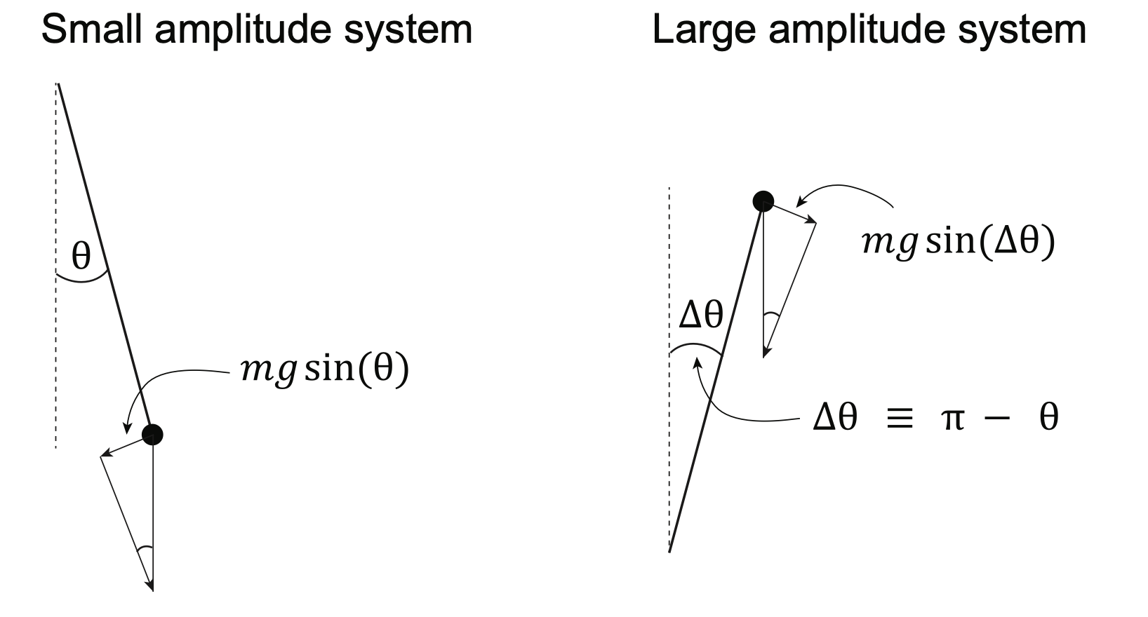
Figure 1. (left) At small amplitudes, the torque on the pendulum can be approximated as \(\tau = -m g L \sin \theta\) \(\sim - mgL \theta,\) where \(L\) is the pendulum's length. (right) For small \(\Delta \theta \equiv \pi -\theta\), the torque \(\tau \approx m g L \Delta \theta\).
Small angle approximation
To begin, we'll review the small amplitude approximation. The left side of Figure 1 illustrates the system in question. To characterize the motion here, recall Newton's second law of rotation,
\begin{eqnarray} \tau = I \alpha \tag{1} \label{tia} \end{eqnarray}
Here, \(\tau\) is the torque, \(I\) is the moment of inertia, and \(\alpha\) is the angular acceleration. Plugging in the relevant expressions for the pendulum, we obtain the equation of motion
\begin{eqnarray} \ddot{\theta} = -\frac{g}{L} \sin(\theta) \tag{2} \label{pita} \end{eqnarray}
Now at small amplitudes, we can apply the approximation \(\sin(\theta) \approx \theta\) to obtain
\begin{eqnarray} \ddot{\theta} \approx -\frac{g}{L} \theta \tag{3} \label{small} \end{eqnarray}
which has solution
\begin{eqnarray} \theta = A \sin \left (\sqrt{\frac{g}{L}} t + \phi \right) \tag{4} \label{sol_small} \end{eqnarray}
Here, \(A\) is the amplitude and \(\phi\) is a constant phase shift. The solution (\ref{sol_small}) is oscillatory, with period
\begin{eqnarray} T = 2 \pi \sqrt{ \frac{L}{g}} \tag{5}\label{period_small} \end{eqnarray}
This is the familiar result. Next, we'll consider the large-amplitude limit.
Large angle approximation
At large amplitudes, the period is dominated by time spent near the upper vertical, as in the right side of Figure 1. To highlight that region, we'll write
\begin{eqnarray} \Delta \theta \equiv \pi - \theta \tag{6} \label{dtheta} \end{eqnarray}
and plug into (\ref{pita}) to obtain
\begin{eqnarray} \Delta\ddot{ \theta} = \frac{g}{L} \sin (\Delta \theta) \tag{7}\label{pita_la} \end{eqnarray}
Close to the upper vertical, we can then again apply a small angle approximation, writing
\begin{eqnarray} \Delta \ddot{ \theta} \approx \frac{g}{L} \Delta \theta \tag{8}\label{eom_la} \end{eqnarray}
The solutions to (\ref{eom_la}) are now exponential rather than sinusoidal,
\begin{eqnarray} \Delta \theta \sim \Delta \theta_0 \exp\left ( \sqrt{ \frac{g}{L}} t \right) \tag{9}\label{la_sol} \end{eqnarray}
Here, \(\Delta \theta_0 \equiv \pi - \theta_{max}\) and we've neglected an exponentially decaying term for simplicity. This form (\ref{la_sol}) will hold up until the point that the angle is so large that our small angle approximation to (\ref{pita_la}) is no longer accurate. This will occur at some finite angle \(\Delta \theta^*\) that does not depend on \(\theta_{max}\). The time that it takes to reach that point can be obtained from (\ref{la_sol}), which gives
\begin{eqnarray} \frac{\Delta \theta^*}{\pi - \theta_{max}} = \exp\left( \sqrt{ \frac{g}{L}} t \right) \tag{10} \end{eqnarray}
Solving for \(t\) and noting that in a full period there are four "swings" through this dominating region (one each on the way up and down on the right, and two more on the left near \(\theta \sim - \pi\)), we obtain
\begin{eqnarray} T \sim 4 \sqrt{\frac{L}{g}} \log \left (\frac{8}{\pi - \theta_{max}} \right) \tag{11} \label{period}. \end{eqnarray}
Here, the factor of \(8\) in the logarithm provides a constant correction to the period. We can't derive this second-order constant correction term using our simple argument here, but may revisit this in a follow-up post. Figure 2 illustrates the correctness of the expression (\ref{period}) for large amplitudes.
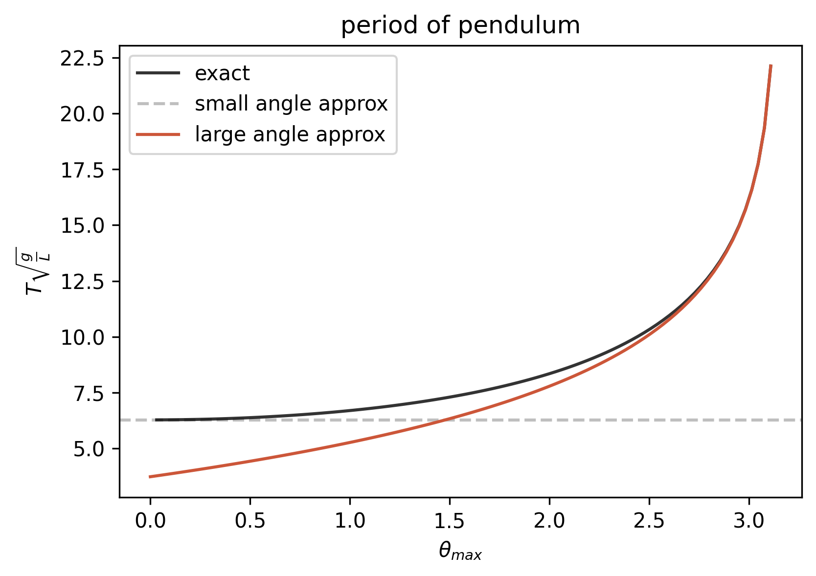
Figure 2. The period of the pendulum vs. \(\theta_{max}\), comparing the approximation (\ref{period}) to the exact result.
References
Similar derivations to ours can be found in [1] and [2].
[1] E. Butikov, “Oscillations of a simple pendulum with extremely large amplitudes,” European Journal of Physics 33, 1555–1563 (2012).
[2] Sanjoy Mahajan in Street-Fighting Mathematics, Problem Set 2 Solutions, Problem 6 (MIT OpenCourseWare, 2008).