Python 3.15 的超低开销解释器分析模式

Python 3.15 的超低开销解释器分析模式 – Ken Jin 的博客
Python 3.15's Ultra-Low Overhead Interpreter Profiling Mode – Ken Jin's Blog

原始链接: https://fidget-spinner.github.io/posts/ultra-fast-tracing.html

Python 3.15 引入了一种新型、低开销的解释器性能分析方法，以支持其新的即时（JIT）编译器。传统的性能分析通常要么需要维护两个独立的解释器（导致代码臃肿），要么需要增加条件性的“分析模式”分支（降低执行速度），而 CPython 3.15 采用了“双重调度”（Dual Dispatch）技术。通过维护两个调度表（一个用于执行，一个用于分析），解释器只需在运行时交换变量即可切换模式，从而避免了昂贵的分支指令。关键在于，分析表将所有指令汇聚到一个单一的记录处理程序中，然后由该程序分派给标准解释器进行执行。这种“扇入/扇出”方式与传统的元追踪系统相比，显著降低了性能损耗。基准测试显示，该方法仅带来约 4.5 倍的开销，相较于其他可能导致近 1000 倍减速的追踪实现，有了显著改善。尽管作者指出该系统增加了复杂性，但它为运行时性能分析和 JIT 追踪记录提供了一个强大且高效的基础。

Hacker News 最新 | 过往 | 评论 | 提问 | 展示 | 招聘 | 提交登录 Python 3.15 的超低开销解释器性能分析模式 – Ken Jin 的博客 (fidget-spinner.github.io) 9 分 | rbanffy 发布于 2 小时前 | 隐藏 | 过往 | 收藏 | 讨论 | 帮助考虑申请 YC 2026 秋季班！申请截止日期为 7 月 27 日。准则 | 常见问题 | 列表 | API | 安全 | 法律 | 申请 YC | 联系搜索：

原文

1 July 2026

Python’s 3.15 JIT shows modest speedups over the interpreter. Key to that is a (to the best of my knowledge), new form of interpreter profiling that was developed for recording execution through the interpreter for JIT compilation. This form of profiling does not introduce much overhead over the interpreter as well, allowing for low-overhead JIT compilation. I wouldn’t be surprised if someone actually already came up with this before, but as far as I could find, it’s not documented anywhere.

Brief Background

In an earlier post, I explained trace recording in the CPython 3.15 JIT. The key idea is that we record an instruction stream through actual program execution, until we hit some terminating condition, then we send that for JIT compilation. Naturally, this requires an instrumented/profiled interpreter.

Profiling an Interpreter

There are normally two avenues of profiling an interpreter:

Have two bespoke interpreters (one for execution and one just for profiling).
Implement a “profiling mode”.

Approach 1: Two Interpreters

Two interpreters, one execution, one profiling, and arrows connecting the two.

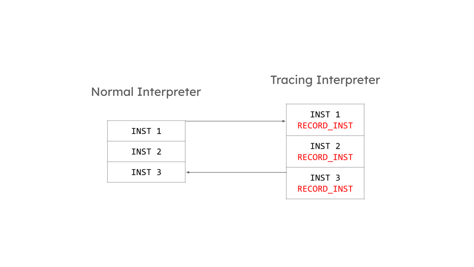
The normal interpreter will have points calling into the profiling interpreter, and a way for the profiling interpreter to return into the normal interpreter. This allows switching back and forth between interpreters. This was the initial implementation of trace recording in CPython. I found it to be alright for the tail-calling interpreter but too slow for the computed goto interpreter (roughly a 6% slowdown on pyperformance!). I suspect the main reason was that we doubled the size of the actual interpreter implemented in C effectively for computed gotos, as that feature is function-scoped. Doubling the size of your C binary is usually not good for performance for various reasons.

Approach 2: Profiling Mode

Profiling mode interpreter

The other common way to implement a profiling interpreter is to have a “profiling mode” which conditions some profiling logic on a boolean, say bool profile. While this minimizes the code bloat, we deemed it too disruptive to the normal interpreter and it would also slow down execution despite the branch being almost always correctly predicted by CPUs.

Dual Dispatch

To get the best out of both worlds, there is one last alternative—swap out the dispatch tables.

Dual dispatch interpreter, showing a normal interpreter with arrows showing how control-flow alternates between normal execution and profiling mode.

Interpreters often dispatch to the next instruction by mapping the opcode (instruction ID) to a function pointer/label address. This tells the interpreter where to go for each instruction.

The idea instead here is to have two dispatch tables—one for normal execution, and one for the profilinng interpreter. At runtime, we just need to assign a local variable dispatch_table_var to decide what “mode” we are in. No branches needed! I’m quite sure I’m not the first person to do this. However, the naiive implementation of this actually gets code that is equivalent to two interpreters in one, which as I wrote above, is very slow. The key improvement then is to map all the instructions in the second table to a singular recording/profillng instruction. This instruction then does all profiling we need, and dispatches using a fixed first table to the actual next instruction in the normal interpreter for execution. You can think of this as a fan-in (to a single instruction) fan-out model. Entering profiling mode is just initializing our data structures, and interpreter wise it’s just swapping out the dispatch tables! Leaving profiling is once again, finalizing our data structures and swapping out the dispatch tables. This is the actual code in CPython 3.15:

#  define ENTER_TRACING() \
    DISPATCH_TABLE_VAR = TRACING_DISPATCH_TABLE;
#  define LEAVE_TRACING() \
    DISPATCH_TABLE_VAR = DISPATCH_TABLE;

The macros are just to handle the different tables when using comupted goto/tail calling interpreter.

Results

Turning off dynamic frequency scaling on my system and running a test script (found in the Appendix), these are the medians of 40 runs measuring the overhead of profiling the interpreter:

# No profiling (just interpreter)
1.72e-06s
# Interpreter + Profiling + JIT compilation
7.47e-06s

This essentially means profiling the interpreter in CPython 3.15 is only at most 4.5x slower for our toy benchmark! Other tracing systems like PyPy have slowdowns in the range of 900x-1000x ! This is of course, not a fair comparison, as PyPy is meta-tracing and thus naturally traces a lot more code than us for the same program (it has to trace the interpreter itself). However, I just put this here to give an example of how slow tracing can actually be.

Reflections

I’m very proud of what we managed to come up with for the profiling interpreter. This approach is not restricted to just trace recording. Other applications might be to introduce low-overhead profiling of an interpreter without radical rewrites, or recording an interpreter’s type profile seen during runtime, etc. Part of why I’m writing this blog post is that I believe in documenting technical knowledge and sharing it in case someone finds it useful. However, I do ask myself ocassionally: is this magical system we’ve come up with in CPython worth the complexity? I like systems that are elegant and simple, and this while elegant is definitely not that simple to reason about. I’ll pen down my thoughts on tracing more in the future..

Appendix

The benchmarking script to measure the overhead. To trigger JIT compilation, I use PYTHON_JIT_RESUME_INITIAL_VALUE=1:

def foo(x):
    x + x
    x + x
    x + x
    x + x
    x + x
    x + x
    x + x
    x + x
    x + x
    x + x
    x + x
    x + x
    x + x
    x + x
    x + x
    x + x
    x + x
    x + x
    x + x
    x + x
    x + x
    x + x
    x + x
    x + x
    x + x
    x + x
    x + x
    x + x
    x + x
    x + x
    x + x
    x + x
    x + x
    x + x
    x + x
    x + x
    x + x
    x + x
    x + x
    x + x
    x + x
    x + x
    x + x
    x + x
    x + x
    x + x
    x + x
    x + x
    x + x
    x + x
    x + x
    x + x
    x + x
    x + x
    x + x
    x + x
    x + x
    x + x
    x + x
    x + x
    x + x
    x + x
    x + x
    x + x
    x + x
    x + x
    x + x
    x + x
    x + x
    x + x
    x + x
    x + x
    x + x
    x + x
    x + x
    x + x
    x + x
    x + x
    x + x
    x + x
    x + x
    x + x
    x + x
    x + x
    x + x
    x + x
    x + x
    x + x
    x + x
    x + x
    x + x
    x + x
    x + x
    x + x
    x + x
    x + x
    x + x
    x + x
    x + x
    x + x
    x + x
    x + x
    x + x
    x + x
    x + x
    x + x
    x + x
    x + x
    x + x
    x + x
    x + x
    x + x
    x + x
    x + x
    x + x
    x + x
    x + x
    x + x
    x + x
    x + x
    x + x
    x + x
    x + x
    x + x
    x + x
    x + x
    x + x
    x + x
    x + x
    x + x
    x + x
    x + x
    x + x
    x + x
    x + x
    x + x
    x + x
    x + x
    x + x
    x + x
    x + x
    x + x
    x + x
    x + x
    x + x
    x + x
    x + x
    x + x




foo(1)
foo(1)
foo(1)
import sys
import time
start = time.time()
foo(1)
end = time.time()
print(end - start)
# sys._dump_tracelets("hello.gvz")