Blog post by Clément Jambon.

1Elliptic PDEs and Boundary Value Problems

Many real-world phenomena are governed by elliptic partial differential equations (PDEs): heat conduction, electrostatics, path planning, steady-state potential flow, and more. These are often cast as boundary value problems (BVPs), where values are prescribed on the boundary of a domain and we seek the solution to the PDE in the interior.

Consider for example the Laplace equation with Dirichlet boundary conditions:

$$ \begin{cases} \Delta u = 0 & \text{in } \Omega \\ u = g & \text{on } \partial\Omega_D \end{cases} $$

Feel free to play with the interactive figure below to get an intuition for what this does:

We can make things more interesting by considering more complex geometries and boundary conditions. For example, people are often interested in solving mixed boundary value problems with Neumann boundary conditionsNote that we will restrict ourselves to zero-Neumann conditions.:

$$ \begin{cases} \Delta u = 0 & \text{in } \Omega \\ u = g & \text{on } \partial\Omega_D \\ \frac{\partial u}{\partial n} = 0 & \text{on } \partial\Omega_N \end{cases} $$

The interactive figure below illustrates this. Notice how the isolines bend to meet the zero-Neumann obstacle at right angles to satisfy $\frac{\partial u}{\partial n} = 0$.

If you look closely, you'll see that the solution is actually "pixelated". This is because it is computed with finite differences on a grid. Finite differences are very easy to understand and to implement but they don't deal very well with complex geometries, often requiring extreme grid refinement. Another common alternative is to use finite elements. The problem is that finite elements require careful mesh generation, which can be particularly challenging and time-consuming for complex geometries Imagine designing a car and having to regenerate the mesh every time you tweak the design. That would be a nightmare — and it is! , such as the city shown below.

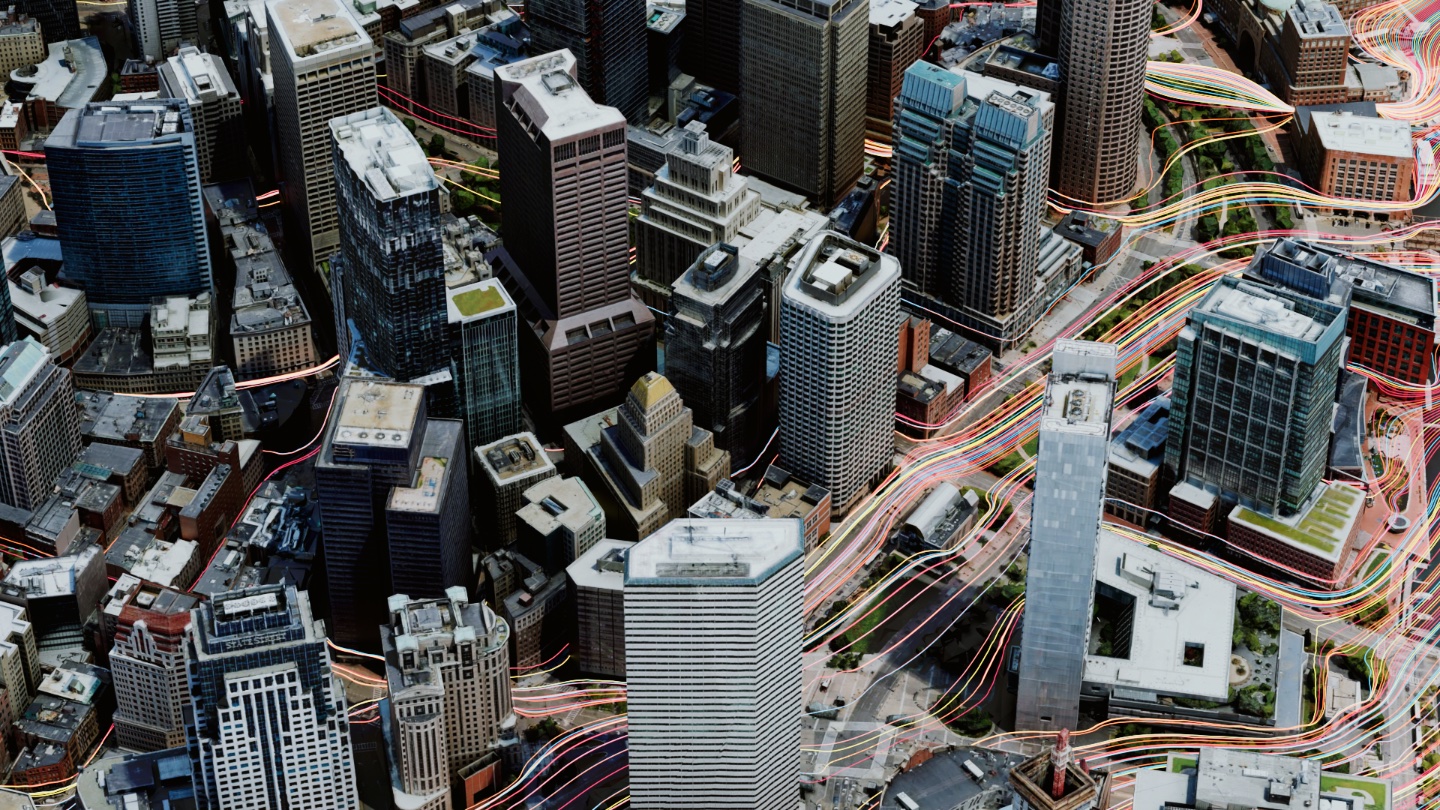
Wind around a city. This scene contains hundreds of buildings with intricate geometry. Our method characterizes their influence on wind patterns, visualized here as steady-state potential streamlines.

2Grid-Free Monte Carlo Methods

Luckily, the computer graphics community has recently revived an old idea: grid-free Monte Carlo methods. The canonical algorithm underpinning this approach is the Walk on Spheres (WoS) algorithm.

The intuition, from stochastic calculus, is that if you were to simulate a Brownian motion (a continuous random walk) starting from an interior point $x$, it would eventually hit the boundary at some random location $Z_\tau$. The expected value $\mathbb{E}[g(Z_\tau)]$ of the boundary condition at that random location is exactly the solution to the Dirichlet problem given by .

However, simulating Brownian motion is computationally expensive and often biasedYou typically have to discretize it, for example with fixed time steps with Euler–Maruyama.. The Walk on Spheres algorithm overcomes this by observing that the exit distribution of Brownian motion on a sphere is exactly uniform. This lets us instead hop from one sphere boundary to the next, where each sphere is inscribed in the domain and chosen to be as large as possible to converge fasterSince walks cannot reach the boundary exactly, we introduce a thin $\epsilon$-shell around it where walks are absorbed when they reach it..

The entire process is illustrated in the interactive figure below. For Neumann boundary conditions, it turns out that there is a special variant of WoS called Walk on Stars (WoSt)As its name suggests, this method "walks on stars" to better handle Neumann (reflective) boundary conditions. Note that from the interactive figure below, it isn't so obvious. The reason is that with rectangles, due to corners, star-shaped domains look basically like slices of a sphere.. If you're interested in learning more about Monte Carlo methods for PDEs, there's a great course and resources available here.

Monte Carlo methods are truly magic! However, as you can see by playing with the interactive figure above, random walks take a lot of steps before they hit the boundary. This is particularly true for problems with complex geometries and Neumann-dominated boundariesOur manuscript showcases a lot of these examples: the warehouse in Figure 1, the city in Figure 4 or the maze in Figure 15.. The main consequence is variance and slow convergence, which render them quite impractical for scenarios where reliable solutions are requiredAnd I believe this may be why people have been hesitant to adopt these methods in practice..

In our work, we address this issue in two complementary waysI should add that we're not the first to tackle this problem. There have been many ways of solving it. The key contribution and novelty of our approach is that rather than simply improving the efficiency of Monte Carlo estimators or caching solutions, we propose a way to connect grid-free Monte Carlo methods with deterministic grid-based solvers, and leverage the nice properties of the latter. . First, as shown in , we can make walks shorter by decomposing the domain into smaller subdomains. Second, as introduced later in , we can "kill" variance, at the cost of a (controllable) discretization bias, by coupling all subdomains together with a deterministic solver, recovering the nice "variance-free" properties of deterministic grid-based methods.

First, observe that a beautiful property of $\Delta u = 0$ in is that this holds everywhere, including on subdomains of the entire domain $\Omega$. As such, a key intuition is that walks can naturally be made shorter by decomposing the domain into smaller subdomains.

Within a single tile $\Omega_i$, is also satisfied, so knowing the boundary values fully determines the interior solution. Concretely, we can encode this as a linear operator $\mathcal{H}_i$ that maps boundary values to interior values:

An absorbing Markov chain is also a random walk, but this time on a discrete (and finite) set of states $\mathcal{S}$. Some states $\mathcal{T}$ are called transient (the walker may pass through them, possibly many times) and the rest $\mathcal{A}$ are absorbing (once entered, the walker never leaves), such that $\mathcal{S} = \mathcal{T} \sqcup \mathcal{A}$. The figure below provides a simple example.

A key observation is that we can also define a boundary value problem on the absorbing Markov chain analogous to . Concretely, as shown in the interactive example below, we can prescribe values on absorbing states, run walks from transient states until they are absorbed, and average the absorbing values to get a solution defined on the transient states, i.e., $$u(t) = \mathbb{E}[g(A_\tau) \mid X_0 = t]$$ for any transient state $t \in \mathcal{T}$, where $A_\tau \in \mathcal{A}$ is the absorbing state where the walk ends and $g$ holds the prescribed values at absorbing states. This is very reminiscent of the Walk on Spheres algorithm, isn't it?

Look at any transient state $i$. By the memoryless property of Markov chains, a walker sitting at $i$ takes a single step to a neighbor $j$ with probability $P_{ij}$, and from there the rest of the walk is statistically identical to a fresh walk launched at $j$. In other words, the expected absorbed value at $i$ is just the weighted average of the expected absorbed values at its neighbors:

$$ \begin{aligned} u(i) &\;=\; \sum_{j \in \mathcal{S}} P_{ij}\, u(j) && \text{on } \mathcal{T}, \\ u(a) &\;=\; g(a) && \text{on } \mathcal{A}. \end{aligned} $$

This is exactly a discrete analog of the Laplace equation : each interior value is the average of its neighbors, with prescribed values on the boundaryIn the continuous case, this mean-value property is locally captured by the Laplacian operator being zero. But note that it also holds in an integral sense as $u(x) = \frac{1}{|\partial B(x, R)|}\int_{\partial B(x, R)} u(z)\,dz$ for a ball centered at $x$ of radius $R$.. Random walks have quietly disappeared: we're left with a system of linear equations where the unknowns are the transient values.

One last fun thing for the road! It turns out that you can see $\mathbf{I}-\mathbf{P}$ as a random-walk Laplacian. In 1D, if we choose a symmetric random walk, the corresponding random-walk Laplacian should be very familiar to you: it's exactly the three-point finite difference Laplacian in 1D (up to a scaling factor).

And in 2D, the random-walk Laplacian for a symmetric walk on a regular grid recovers the standard five-point finite-difference stencil.

From there, you probably see the pattern. What if instead of these canonical probabilities, we considered more general transition probabilities based on the geometry of the subdomains?

6Coupling Tiles via an Absorbing Markov Chain

Now we have almost all the pieces to recover values at interfaces between subdomains! The trick is to Walk on Decomposed Subdomains, or more precisely on their interfaces.

The last problem is that, so far, we've only seen in how to jump from the inside of a subdomain to one of its interfaces and not from one interface to another. The fix is to view each interface through another decompositionThis time it is an overlapping decomposition. of the domain, one where the interface sits in the interior of a subdomain. On a grid, that subdomain is just the two cells sharing the edge, and its boundary is made of the neighboring interfaces (or pieces of the global boundary). We call these “co-edge” subdomains.