This article is a deep dive into xorshift generators, one of the most adopted families of algorithms for the generation of pseudorandom numbers.
This is a companion article to a video documentary which will be released in the following weeks.
If you want to learn more about xorshift generators, including tables of maximal triplets, you can consult the Xorshift: Appendix.
Introduction
At this very moment, billions of devices are running these three lines of code.
uint64_t x;
uint64_t y;

uint64_t next()
{
	uint64_t t = x;
	const uint64_t s = y;
	x = s;
	t ^= t << 23; // a
	t ^= t >> 17; // b
	t ^= s ^ (s >> 26); // c
	y = t;
	return t + s;
}
They hide inside virtually every browser, and the servers they talk to.
They control the events that happen while you’re playing. From the worlds you explore, to the cards in your hand.
This algorithm—and the others like it—are the metaphorical dice that your computer rolls every time it makes a decision. But …what does it do, and how does it work?
I’m Alan Zucconi, and in this documentary we’ll travel to the very source of randomness, by dissecting the most popular family of pseudorandom algorithms: xorshift generators.
And we’ll do it by asking a very simple question: what makes 23, 17 and 26 special?
Part 1: Xorshift Generators
Pseudorandom numbers
Computers are terrible at being random. In fact, every “random” number you have ever generated was almost certainly completely deterministic.
But it turns out that with the right algorithm, deterministic sequences can look random enough to power games, simulations, procedural content, cryptography—well, okay, maybe not cryptography …but we’ll get back to that later.
Most of these pseudorandom techniques work on the same principle: there’s a function that we apply to the previous number in the sequence, to get the next one. The first one—the seed—is given, and the rest of the sequence follows from it.
That’s how games like No Man’s Sky and Minecraft are able to “compress” entire galaxies and worlds in a number. That’s the seed that kickstarts the sequence of pseudorandom numbers, and with the same seed, you get the same sequence. If you are curious to find out more about this, I made an entire documentary about the world generation of Minecraft.
Marsaglia’s Xorshift
In 2003, mathematician George Marsaglia published a short paper (“Xorshift RNGs“) introducing a family of generators that fall into this category, based almost on two operations: XOR and shifts. Unsurprisingly, they’re called xorshift generators.
This one here, for example, generates sequences of 32-bit numbers:
uint32_t x;
uint32_t xorshift32(void)
{
	x ^= x << 13;
	x ^= x >> 17;
	x ^= x << 5;
	return x;
}
📝 Variable types used by Marsaglia
In his original paper, Marsaglia’s code used unsigned long for the variables. In C/C++, the size of types depends on the platform. In his case, unsigned long is 32 bits, and unsigned long long is 64 bits.
To avoid confusion, in this article we used uint32_t and uint64_t. If you are implementing this in C#, you can use uint and ulong, respectively.
The original paper published by Marsaglia contained a typo. The xorshift32 code on page 4:
unsigned long xor(){
static unsigned long y=2463534242;
yˆ=(y<<13); y=(y>>17); return (yˆ=(y<<5)); }
Should have been instead this:
unsigned long xor(){
static unsigned long y=2463534242;
yˆ=(y<<13); y^=(y>>17); return (yˆ=(y<<5)); }
There are 8 possible variants of this code:
If a triplet  is maximal for one of those, it is also maximal for the other seven (although the overall sequence might exhibit different statistical properties).
Let’s see how it works, line by line!
It takes the previous number in the sequence (x), makes a copy, and shifts its bits 13 times to the left. It drops the bits that overflow, and fills the rest with zeros.

left shift x << 1

right shift x >> 1
Now: every time there’s a “1”, it flips the corresponding original bit: that’s a bitwise XOR.
Next, it does another xorshift: copy, shift, XOR. But this time, shifting by 17 bits to the right. And once more, by 5 bits to the left.

No multiplications. No divisions. No lookup tables. Just a few bitwise instructions. If we paint a texture using these values as colours …well, it looks pretty random to me!
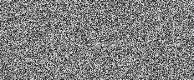
But why did Marsaglia himself recommend shifting by 13, 17, and 5 bits? Why not 42, 67, and 1729? And why exactly three xorshift operations, and not two, or four?
It’s questions like these that you should always ask when you see magic numbers in someone else’s code. Like 0x5F3759DF from Quake’s Fast Inverse Square Root function, or the golden ratio constant 0x9e3779b97f4a7c15 found in a lot of hashing algorithms.
These constants might be arbitrary, but they’re never random. Because they almost always reveal something deeper about the problem, and the way in which it was solved.
So… what happens if we try a different triplet!?
These sequences don’t look that random anymore! And that’s because the period of most triplets—which is, how many unique numbers they generate—is far too small to be used for procedural generation!
What makes 13, 17, and 5 special is that it’s a maximal triplet! Out of all the possible ones—that’s  —there are only 162 that generates all 32-bit numbers. Well, all except zero, which xorshifts can never generate anyway.
Over four billion states ( ) from three lines of code.
When a triplet is maximal, the sequence of pseudorandom numbers it generates cycles through all possible non-zero values. This means that changing the seed effectively “shifts” where the sequence starts from.
When the triplet is not maximal, the period is partitioned across smaller cycles. Different seeds will land in one of the many cycles of the generator, but none of them will be maximal.
You can read more about the underlying mathematics in this paper titled “The cycle structure of a linear transformation over a finite field“.
If you’re thinking this works because these (13, 17, and 5) are all prime numbers… well, you’d be wrong! In fact, (2, 15, 25) and (16, 21, 9) work… just as fine!
And if you test all combinations, you’ll also find out that we need 3 xorshifts, because you can’t generate all 32-bit numbers with just two of them!
| shifts \ bits | 32 bits | 64 bits |
|---|---|---|
2 shifts<< a>> b | no solutions | xorshift64 (7, 9) 2 solutions |
3 shifts<< a>> b<< c | xorshift32 (13, 17, 5) 162 solutions | xorshift64 (13, 7, 17) 550 solutions |
In his original paper, Marsaglia indicated there were no maximal tuples for 64 bits. That is not the case, as both (7,9) and (9,7) are maximal.
When visualised in three dimensions, the maximal triplets arrange on a complex structure. Below, you can see the arrangement of the canonical maximal triplets for  .
.
As  gets larger, the structure appears to get denser, not richer. This indicates that the lattice structure of maximal triplets is consistent across different values of .
You can clearly see in the scatter plot above a “line”, emerging from a sequence of aligned maximal triplets.
All points on that line have different matrices which share the same primitive polynomial. Such “primitive lines” appears to lie on the “edges” and “faces” of the three-dimensional structure that emerges from the maximal triplet distribution.
They becomes really abundant when the period is a Mersenne prime.
Finding triplets
But how do we find those maximal triplets? The most naïve way is to count how many unique numbers each one generates. With 32 bits we have almost 30.000 triplets to check ( ), and each one generates up to almost 4.3 billion unique numbers (
 ). Which is… a lot, but nothing we can’t test in a few hours!
So what about 64-bit numbers? You may think that doubling the number of bits, also doubles the search time. But that would be …incorrect! It is every new bit that doubles the range of numbers we can represent. So going from 32 to 64 bits actually doubles the range—and the search time—32 times! That’s roughly …49 million years. Give or take.
So how could Marsaglia do this—in minutes—back in 2003? Well, he did it with two very clever tricks…
❓ The Hull-Dobell Theorem
Part 2: Matrix Approach
Underneath their code, xorshift generators are secretly just matrix multiplications:
(2) 
And this matters, because Linear Algebra can predict the length of a sequence, without calculating all of its elements.
Let’s treat the bits of our seed as the components of a vector. Every instruction in our code translates to a linear transformation between vectors and matrices. That’s our first trick, and it’s not a coincidence: the algorithm is literally designed like this to make the search for maximal triplets feasible.
Vectors can be represented in two separate notations: either as rows or columns.
Marsaglia used the row vector notation:

Other authors are using the column vector notation instead:

The latter can be quite inconvenient to write inline, as it effectively breaks the layout (like this:  ).
).
Some authors express inline column vectors as row vectors, using the transpose operator:  .
.
While this merely represents a preference, it changes how equations are written. Due to the way matrix multiplication works, it holds that:

row vectors must be multiplied from the left; column vectors from the right:
In row vector notation, matrix multiplications are written as  ; in column vector notation, they are written as
  instead.
Bitshifts
You probably already know that when a vector is multiplied by the identity matrix, it remains unchanged.
(3) 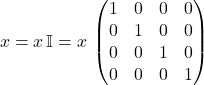
This happens because matrix multiplication is defined in such a way that the positions of the 1s in each column define which bits are linearly combined to produce the output vector.
Shifting the diagonal down shifts the output bits to the left. Let’s call this matrix  !
!
(4) 
If we want to shift by two bits (x << 2), we multiply the result by once more!
And because multiplication is associative, it turns out that to shift a vector by  bits (
x << a), we multiply it by raised to the  -th power.
(5) 
And the exact same reasoning holds for a right shift (x >> a), which is equivalent to  :
:
(6) 
Xor
The bitwise XOR (between two variables) happens to behave exactly like the component-wise addition (between two vectors).
And since all those vectors contain either zero or one, let’s say that 1+1=0. You can think about this as “addition without carry over”, or “addition followed by modulo 2”. But—for the hardcore fans of Field Theory—that’s simply a finite field with two elements.
❓ Finite field with two elements
You are surely familiar with addition and multiplication between integer numbers. Their set,  , has infinitely many elements. In contrast, a finite field only has a finite number of elements. In the case of a finite field with two elements, that means restricting to only two elements: 0 and 1. It is referred to as
  (where
  stands for field), or
  (where
  stands for Galois Field).
Under normal conditions, you would expect  . But in , there is no concept of “2”. Addition on a finite field is defined in a slightly different way, which makes numbers “loop”. So,
  . You can think about as operating on , but applying a modulo 2 after every operation:

This is why the field is also referred to as  (or simply
  ), which is the system of integers modulo 2.
If the idea that still sounds nonsensical, you can think about binary numbers (which are represented with two digits only), where  . If we only focus on the right-most bit, it is indeed true that . That’s like addition without carry-over.
❓Galois Fields and Boolean Algebra
❓ Galois field and prime numbers
❓ Galois Fields: GF(2), GF(2)ⁿ, and GF(2ⁿ)
Xorshift
We now have everything we need to express one single xorshift operation (x ^ (x << a)) in its matrix form:  .
.
And if we want to perform three of them in series, we just multiply the original number by three separate matrices!
That’s our final matrix  , and it looks like this:
(7) 
It is important to remember that those are binary matrices: every cell can only contain zero or one. This means that we can visualise them as bitmaps:


And when we do that, the matrix looks like this:

🟰 Show me the derivation

Part 3: Order Test
Now that the xorshift is framed in terms of vectors and matrices, we can take advantage of Linear Algebra. The period of a generator—which is, how many unique numbers it produces—corresponds to the multiplicative order of its matrix.
That is defined as the smallest value  for which
  :
:
(8) 
Hence, a triplet is maximal if and only if that multiplicative order is equal to all the possible non-zero numbers that can be represented with  bits:
bits:
(9) 
Let’s see what all of this means in practice.
Each time we multiply by , we progress in the sequence.
(10) 
which means that:
(11) 
Matrix multiplication is associative, so we can group all the s together. The -th element of the sequence is found by multiplying the first one by  , skipping all the intermediate ones!
(12) 
After a certain number of iterations—let’s call it  for period—we get back to the starting element, and the sequence repeats:
(13) 
Since  is guaranteed to be non-null (as xorshift generators can never produce 0), we can simplify the s on both sides, and find out that if a sequence repeats after iterations, then
  is the identity matrix! Let’s call this the identity test.
Maximal Order test
Now, if a number p passes the identity test, it doesn’t necessarily mean that’s the actual period of our sequence! If numbers repeat after 30 iterations; they’ll also repeat after 60, after 90, after 120 …because it’s like looping through the sequence two, three, four times…

In a nutshell, if passes the identity test, so do all of its integer multiples  (with
(with  ):
):
(14) 
This also means that if 30 passes the identity test, perhaps that’s because the actual period is 15 and we just looped twice! Or perhaps it was 10, and we looped 3 times. Or it was 6, and we looped 5 times!

You get where I’m going with this: for 30 to be the smallest period, none of its divisors should pass the identity test—including 5, 3, and 2.
In fact, (\eq{Tn_eq}) also implies that if a number doesn’t pass the identity test, then none of its proper divisors will:
(15) 
But we don’t have to test them all! 15 is 5 times 3: if 15 doesn’t pass the identity test, neither 5 nor 3 do! If 10 doesn’t pass the identity test, neither 5 nor 2 do. And the same for 6!

So what’s the minimum number of divisors to test?
Well, the prime factors of 30 are 2, 3, and 5; and its divisors are combinations of them.
Testing larger numbers first helps prune more divisors out, so we can remove one prime factor at a time from 30, and those are the minimum number of tests that covers all other cases.

Going back to our original 64bit problem: for a triplet to have period  , itself must pass the identity test, while that same test must fail when we divide by each of its prime factors.

That reduces the number of iterations from 127–all possible divisors including itself–to just 8!
There are 127 divisors (126 if we exclude the original number itself) of  .
.
This can be calculated by counting its prime factors: 7. Every divisor is a combination of those 7 factors, and each combination is guaranteed to result in a different number. This is because every number has a unique prime factorisation, so it is impossible for two combinations of primes to produce the same number.
Counting the factors can be seen as a combinatorial problem. Take up to 6 elements out of a list of 7: 126:

Or 127 if we take up to 7 elements out of 7 (which includes the original number as well):

The number of proper divisors (126) can also be calculated imagining that, for every factor, we can either choose it or not chose it. There’s a total of  combinations, from which we remove the empty set (zero) and the full set ( itself), resulting once again in 126.
That’s the second trick! And that’s how we find that with 64 bits, we have 550 maximal triplets. With Marsaglia choosing 13, 7 and 17.
Factoring large number is computationally very expensive, and that is definitely the case for  .
.
Luckily for us, numbers of the format  are known as Mersenne numbers, and have been studied extensively in the search for large primes.
Mersenne numbers are strongly connected to Fermat numbers, which are of the form:
(16) 
The product of the first Fermat numbers is equal to:
(17) 
This means that as the prime factorisation of more and more Fermat numbers is discovered, more numbers of the form  can be factorised.
That is the the subset of all Mersenne numbers which exponent is a power of two (such as  ,
,  ,
,  , and so on).
Right now, only the prime factorisation of the first 12 Fermat numbers is fully known. This means that (using the order test) we can only find all maximal triplets with absolute certainty only up to  .
.
Higher values of might be testable, providing that the prime factorisation of is known.
🟰Prime factorisation of Fermat numbers
Part 4: Companion Matrices
We’ve done 32 bits… we’ve done 64… what about 128?
Our algorithm finds 1072 full-period triplets, but none of them can be found in the selected list presented by Marsaglia: (11, 8, 19), (5, 14, 1), (15, 4, 21), (23, 24, 3), and (5, 12, 29).
What’s going on? Well, modern architectures natively support bitwise operations with 32 and 64 bits. But that’s not typically the case for 128, making a “true”, “monolithic” xorshift128 neither efficient to run, nor elegant to write.
📄 Monolithic xorshift128 code
Below, a version of a monolithic xorshift128 built using four 32-bit variables:
uint32_t x;
uint32_t y;
uint32_t z;
uint32_t w;

uint32_t next()
{
	uint32_t tx, ty, tz, tw;

	// s ^= s << a
	tx = (x << a) | (y >> (32-a));
	ty = (y << a) | (z >> (32-a));
	tz = (z << a) | (w >> (32-a));
	tw = (w << a);

	x ^= tx;
	y ^= ty;
	z ^= tz;
	w ^= tw;

	// s ^= s >> b
	tx = (x >> b);
	ty = (y >> b) | (x << (32-b));
	tz = (z >> b) | (y << (32-b));
	tw = (w >> b) | (z << (32-b));

	x ^= tx;
	y ^= ty;
	z ^= tz;
	w ^= tw;

	// s ^= s << c
	tx = (x << c) | (y >> (32-c));
	ty = (y << c) | (z >> (32-c));
	tz = (z << c) | (w >> (32-c));
	tw = (w << c);

	x ^= tx;
	y ^= ty;
	z ^= tz;
	w ^= tw;

	return w;
}
This version only works for shifts up to 31, because it assumes that bits can only “spill” into the neighbouring variable.
To get around this, Marsaglia proposed a similar but different algorithm: one that still uses bitwise operations, but stores the 128-bit state in four 32-bit integers: x, y, z, and w:
uint32_t x;
uint32_t y;
uint32_t z;
uint32_t w;

uint32_t next()
{
	uint32_t t;
	t = x ^ (x << 11); // a
	t = t ^ (t >>  8); // b
	x = y;
	y = z;
	z = w;
	w = w ^ (w >> 19); // c
	w = w ^ t;

	return w;
}
📄 Show me the original code
This is the original code presented by Marsaglia:
unsigned long xor128(){
	static unsigned long x=123456789,y=362436069,z=521288629,w=88675123;
	unsigned long t;
	t=(xˆ(x<<11));x=y;y=z;z=w; return( w=(wˆ(w>>19))ˆ(tˆ(t>>8)) );
}
The code was rewritten for clarity.
❓ Returning a partial state
Previous xorshift implementations (such as xorshift32) returned their entire state. Generally speaking, this is not a good idea. Xorshifts are linear recurrences, and exposing their full state allows one to perfectly predict the next number in the sequence.
In contrast, xorshift128 returns only its least significant 32 bits. For any value returned, there are  possible states with matching lower bits. One output does not uniquely identify the full state.
The state of xorshift128 cycles through all non-zero  possible values. But because only the lower 32 bits are returned, it is possible for the same number to appear twice in a row. That is impossible with xorshift32, because (by construction) the sequence it generates cycles through all possible values once before repeating.
Tying to find consecutive repeating numbers by looping through all the values of xorshift128 is infeasible. Instead, we can prove their existence mathematically.
If the current 128-bit state of the generator is a vector  , the next state
  is calculated using the transformation matrix :
  . For xorshift32, that is also the next output. But for xorshift128, only the lower 32 bits are returned.
We can isolate them by using  , a matrix with 128 rows and 32 columns, which looks like the right-most “slice” of the identity matrix
  :
:  .
.
(18) 
Asking for two consecutive numbers to be equal, means resolving for  :
:

We are looking for the (non-zero) solutions of  .
.
The rank-nullity theorem indicates that the number of solutions is  . The rank of
  is the number of linearly independent columns, which is 32. This means that the nullspace contains at least
  states, and since 0 is not part of the xorshift sequence, there are at least
  non-zero states where .
❓ Finding consecutive numbers
Let’s see how this version works!
Lines 10-12 shift the lower 96 bits to the right, while the rest reshuffles x and w into the lower 32 bits.
The auxiliary variable t stores the result of a left xorshift on x, followed by a right xorshift.
w goes through a right xorshift, and the result is xor-ed with t.

We can work backwards to reconstruct the matrix that maps the input state ![\left[x, y, z, w\right]](https://www.alanzucconi.com/wp-content/ql-cache/quicklatex.com-8925f8c8f00551fc6ed32a06d8845282_l3.png "Rendered by QuickLaTeX.com") to the output state
to the output state ![\left[y, z, w \right]](https://www.alanzucconi.com/wp-content/ql-cache/quicklatex.com-ebbf7247740cf09c2cf87cba43fb4755_l3.png "Rendered by QuickLaTeX.com") and a linear combination of
and a linear combination of  and
and  .
.
And that’s what it looks like, both in block matrix form …and in its full glory.
(20) 

This looks dangerously similar to a Frobenius companion matrix—studied in the context of primitive polynomials for their connection to maximal sequences—hence making it a “natural choice” to restrict the search.
Part 5: Characteristic Polynomials
Later papers explored that connection further, ditching Marsaglia’s naïve order test, in favour of more targeted approaches. After all, we don’t need to find all maximal triplets: we just need to find one that’s good. And primitive polynomials have played a key part in that.
Every square matrix is paired with a characteristic polynomial, which is defined as:
(21) 
The symbol  is often used for the variable (instead of the more common ), especially when eigenvalues and eigenvectors are involved. Regardless, the result is a polynomial of degree , which is used to study certain properties of the matrix.
As it turns out, there’s a special connection between the maximality of a triplet, and its characteristic polynomial: its primitivity.
A polynomial is primitive over if any of its roots  is a primitive element of
  . In a nutshell, it means that:
(22) 
It means that integer powers of a root are cycling through all non-zero elements. Which is exactly what the multiplicative order or the matrix captured.
Krylov Space
Testing for the primitivity of the characteristic polynomial is, generally speaking, much more efficient than testing the multiplicative order of the matrix. Matrix calculations are, in fact, expensive: the multiplication of a dense  matrix by a vector has a computational complexity of
  , while multiplying two dense matrices is
  .
.
A “naïve” test for primitivity would first build the matrix , then extract the characteristic polynomial by solving  . All of those steps are very expensive, and would likely counteract any actual speedup when compared to the traditional order test seen before.
What makes this approach feasible, is that we can reconstruct the characteristic polynomial without building its associated matrix . We do that by constructing the so-called Krylov space first, a part of which is then used by the Berlekamp-Massey algorithm to reconstruct the characteristic polynomial.
A Krylov space is built by multiplying a starting vector by a matrix over and over:
(23) 
Normally, this would be expensive as it requires not only the construction of , but also performing a vector multiplication for every element of the space.
For xorshift generators, that is not necessary: the Krylov sequence is nothing more than the sequence of states generated by the pseudorandom algorithm, which is exceptionally fast to compute!
❓ Which vector v to use?
❓ How many vectors to generate?
A constraint on the number of vectors to generate comes from the Berlekamp–Massey algorithm, which uses them to reconstruct the characteristic polynomial.
A fundamental result behind the BM algorithm indicates that if the true linear complexity of the sequence is , then the first  terms uniquely determine the minimal recurrence.
❓ What about xorshift128?
The algorithm just described works for single-word xorshift generators, like Marsaglia’s xorshift32. It cannot be applied, as it is, to variants like Marsaglia’s xorshift128, which only return part of their full state.
The Krylov sequence must include the full generator state, not just the partial output it returns to the caller!
Berlekamp–Massey Algorithm
The sequence is then passed to the Berlekamp–Massey algorithm, an algorithm which reconstructs minimal polynomials from linear recurrent sequences in arbitrary fields.
The minimal polynomial  is not exactly what we’re after, but it’s close! It’s guaranteed to be a divisor of the characteristic polynomial.
From this, we find ourselves in two scenarios:
This means that the BM algorithm either returns the characteristic polynomial, or one of its proper factors (revealing that the original triplet was not maximal). What it cannot do, on its own, it so tell us if a triplet is maximal. We still don’t know if the returned characteristic polynomial is irreducible, let alone primitive.
But once extracted, the characteristic polynomial can be tested for both conditions, using the same order test previously devised for matrices (but applied to polynomials over ):

📝 Maximality and primitivity
Finding if a triplet is maximal started as a coding problem, but is now expressed in terms of vectors and matrices. The following properties are all equivalent statements, but expressed with the language of their own fields:
- Programming: Maximal period for generators
- Linear Algebra: Maximal multiplicative order for matrices
- Field Theory: Primitivity for characteristic polynomials
Because all of these terms are equivalent definitions of the same concept in different fields, this article uses them somewhat interchangeably. Saying that “a triplet is primitive” is mathematically incorrect, because the concept of primitivity is defined on polynomials, not triplets. But it can be naturally extended, with the meaning that it is not the triplet itself being primitive, but the characteristic polynomial of transition matrix associate with it.
Frobenius Companion Matrices
We have learnt in the previous section that a triplet is maximal if its associated characteristic polynomial is primitive. This connection goes both ways: every primitive polynomial represents a linear recurrence from which a generator can be extracted.
Rather than finding maximal triplets by brute force testing their maximality, it is sometimes more efficient to find a polynomial that is known to be primitive, and rebuild its associated matrix.
The simplest way to do that is through Frobenius companion matrices, which we have briefly mentioned before:
(24) 
whose characteristic polynomial is expressed in the following form:
(25) 
The beauty of a companion matrix is that it contains the coefficients of its characteristic polynomial. And if that is known to be primitive, its companion matrix will be maximal.
This is one of the ideas behind Marsaglia’s companion block matrices, which were indeed designed with a similar block structure in mind.
❓ Marsaglia’s companion block matrices are Frobenius companion matrices
That’s correct. The transformation matrix used by Marsaglia looks like a Frobenius companion matrix in its block form:

with  . And the polynomial
  is indeed primitive over (i.e.: it is irreducible, has degree 4, and its roots are primitive elements over
  )!
)!
But we need to remember that in a block matrix, every element itself is a matrix! When expanded, it actually looks like this:

which is not a Frobenius companion matrix!
The ingenuity of Marsaglia lies in the fact that defining a 4×4 Frobenius companion matrix ensures that, at least at the block level, every component of the state eventually occupies every position:
![\begin{equation*} \label{xywz_cycle} \left[x, y, z, w\right] \to \left[y, z, w, x\right] \to \left[z, w, x, y\right] \to \left[w, x, y, z\right] \end{equation}](https://www.alanzucconi.com/wp-content/ql-cache/quicklatex.com-d35eca2817333ab99cb501500aa19635_l3.png "Rendered by QuickLaTeX.com")
📚 Linear-Feedback Shift Registers
In general, the type or generator that arbitrary primitive polynomials are converted into are called linear-feedback shift registers (LFSR), and pretty much like xorshifts, they are linear recurrences.
As an example, let’s take  , which is a primitive polynomial over . Any of its roots have order
  , which are all the non-zero elements of .
We can rewrite  in as
in as  , and replace the s with sequence values:

Now, remembering that addition in GF is equivalent to a bitwise XOR, we get that:

That’s a linear recurrence on a state with 4 elements ![\left[s_n,s_{n+1},s_{n+2},s_{n+3}\right]](https://www.alanzucconi.com/wp-content/ql-cache/quicklatex.com-e9ffb496573cd597b8f2c741fee84dab_l3.png "Rendered by QuickLaTeX.com") , not dissimilar to the one used by Marsaglia for his xorshift128, which goes through the following update process:
, not dissimilar to the one used by Marsaglia for his xorshift128, which goes through the following update process:
![\begin{equation*} \label{lfsr_p4_3} \left[s_n,s_{n+1},s_{n+2},s_{n+3}\right] \; \to \; \left[s_{n+1},s_{n+2},s_{n+3}, s_n \wedge s_{n+1}\right] \end{equation}](https://www.alanzucconi.com/wp-content/ql-cache/quicklatex.com-277c308a20fb6795ab5953f2309c8ae7_l3.png "Rendered by QuickLaTeX.com")

When implemented directly as above, this represents a Fibonacci LFSR.
The other way to make use of the linear recurrence hidden in the primitive polynomial, is to implement a Galois LFSR, which more closely relates to Marsaglia’s original implementation.
Part 6: Testing
Just because a triplet is maximal, it doesn’t mean it’s also… good.
Different full-period sequences have different statistical properties, and not all of them make good random number generators.
When a sequence looks predictable, it produces linear artefacts which can manifest pretty strongly in procedural terrains and textures.
So what separates the good generators from the bad ones? It’s two things mostly: number one, they should be uniformly distributed, so that all numbers have roughly the same chance. And number two: those numbers should be independent of each other, which is really what makes them “unpredictable”—so to speak.
Basically, they have to behave like virtual dice.
One useful way to measure how “well-behaved” a sequence is, is—well—to test it using tools like dieharder or TestU01. They crunch millions of those numbers, and by measuring their distribution, they infer the underlying properties of their generator.
Diehard is a test suite that measures the quality of random number generators. It was developed by Marsaglia himself, and published in 1995 as a CD-ROM.
Dieharder is an improved version, developed by Robert G. Brown. The original version is currently maintained on his website: Robert G. Brown’s General Tools Page.
Dieharder is available as a command on Ubuntu.
A version of Dieharder compiled for Windows can be found on The Internet Archive.
TestU01 is an improved battery of stress tests for random generators, developed by Pierre L’Ecuyer and Richard Simard in 2007.
It contains three famous test batteries:
- Small crush: 10 tests
- Crush: 96 tests
- Big Crush: 106 tests
A version of TestU01 from 2009 is available on L’Ecuyer website. An unofficial github repository can also be found here.
And perhaps that’s how Marsaglia chose (11, 8, 19) for his xorshift128, and not any of the other 46 maximal triplets.
And even though it was published in 2003, this implementation is still very relevant today because it’s the one used by the most popular game engine in the world. Out of the millions of Unity games out there, almost all of them are powered by the three lines of code that makes xorshift128.
So, wouldn’t it be funny if (11, 8, 19) wasn’t actually the best triplet!? And in fact, it isn’t! It’s probably (11, 5, 12), but—to be fair—that might be just marginally better.
Does it mean that Unity should change it? Hell, no! The integrity of so many games depend on the reliability of its generator, so it’s one of those things that can’t really be changed anymore without the risk of breaking thousands of games!
But in fairness, Unity could perhaps offer a number of different algorithms, like Java does with its java.util.random package.
❓ Random number generators used by game engines
Part 7: Beyond Marsaglia’s xorshift
By the early 2000s, Marsaglia’s xorshifts had become incredibly popular. They were tiny.
They were fast. And they had enormous periods.
But their strength—their mathematical elegance, their linearity—turns out to also be their biggest weakness.
Modern statistical test suites don’t just check whether numbers look random. They search for subtle correlations hidden deep inside the sequence. And because xorshifts are completely linear, some of those tests can detect structures that shouldn’t exist in a truly random source.
One solution to this problem was not to change the xorshift algorithm itself, but to apply a non-linear transformation just to its output.
xorshift64*
Back in 2014, Computer Scientist Sebastiano Vigna found himself in need of a better random number generator than the ones he had available at the time. He continued Marsaglia’s work in a paper titled “An experimental exploration of Marsaglia’s xorshift generators, scrambled“, introducing xorshift64*. That’s a traditional xorshift64, with its output multiplied by a constant before being returned:
uint64_t x;
uint64_t next(void)
{
	x ^= x >> 12; // a
	x ^= x << 25; // b
	x ^= x >> 27; // c
	return x * UINT64_C(2685821657736338717);
}
❓ Why 2685821657736338717?
The multiplication constant chosen by Vigna ( ) came from Pierre L’Ecuyer’s research on Linear Congruential Generators (“Tables of Linear Congruential Generators of different sizes and good lattice structure“, page 259), for its empirical property of scrambling bits.
The constant was proposed in a different context, which gave no guarantee about its effectiveness inside xorshift64*. However, it still proved useful for its statistical properties.
The state of the xorshift is not changed, so all the results (and the triplets) found for xorshift64 also apply to xorshift64* as well. However, the multiplication scrambles the output bits enough to pass most dieharder and TestU01 tests.
Technically, that’s a linear operation between integer numbers, but multiplication and additions are not linear operations in Boolean algebra (where our matrices are defined).
As Vigna noted in his paper, the scrambling operation fundamentally changes not just the sequence, but also its statistical properties. While the maximality of a triplet remains unchanged, its quality might not. This means that the “best” triplets for xorshift64 and xorshift64* are likely different.
xorshift128+
In the same year, Vigna also published “Further scramblings of Marsaglia’s xorshift generators“, where he replaced the multiplication with a constant, with the addition between state variables.
He implemented a traditional xorshift128 generator using two 64-bit variables (below, x and y). But instead of returning just one of them, he returned their sum:
uint64_t x;
uint64_t y;

uint64_t next()
{
	uint64_t result = x + y;
	uint64_t t;
	t = x ^ (x << 23); // a
	t = t ^ (t >> 18); // b
	x = y;
	y = y ^ (y >>  5); // c
	y = y ^ t;
	return result;
}
📄 Original xorshift128p code
The original code, using an array instead of two separate variables, and a more condensed form:
uint64_t s[2];
uint64_t next(void)
{
	uint64_t s1 = s[0];
	const uint64_t s0 = s[1];
	const uint64_t result = s0 + s1;
	s[0] = s0;
	s1 ^= s1 << 23; // a
	s[1] = s1 ^ s0 ^ (s1 >> 18) ^ (s0 >> 5); // b, c
	return result;
}
Vigna published his work using (23, 18, 5). The current implementation in the V8 JavaScript engine uses (23, 17, 26) instead (random-number-generator.h).
Once again, the state itself is left unchanged, but the addition effectively “scrambles” the output bits. And with such a simple change, most of the linear artefacts simply vanished. In comparison to xorshift64*, this version does not rely on an extra parameter.
Unbeknownst to him, his xorshift128+ was about to become one of the most widely deployed pseudorandom number generators ever written.
In 2015, Google announced the adoption of xorshift128+ in their V8 JavaScript engine. Chrome, Edge, Safari, Opera, Firefox, and even Node.js; under the hood, they are all running xorshift128p.
It’s hard to get precise numbers, but that’s roughly 4 to 5 billion active devices globally. And that’s not even counting all other xorshift variants out there. Like Vigna’s xorshiro and xoroshiro algorithms (adopted in various forms by the .NET, Java, and Rust ecosystems), or Marsaglia’s xorwow (which powers NVIDIA CUDA’s random engine), or the 1.5 billion devices running Unity games.
The limits of xorshift generators
Even though xorshift generators are pretty much ubiquitous, there are entire applications in which they simply cannot be used. If you know the state, you can predict the rest of the sequence. One number is typically not enough to do that, but observing just a few of them is all you need to crack the next one. It’s this “predictability” that makes them cryptographically unsafe.
After all, linear sequences like these will always exhibit some statistical weakness.
It’s not a matter of “if” they are going to fail tests suits like dieharder or TestU01: it’s a matter of how long before they detect linear artefacts.
For all those applications where quality and safety are not just desired but necessary, stream ciphers like AES in Counter Mode (AES-CTR) or ChaCha20 have effectively solved all the problems we’ve encountered so far. Because they effectively provided the cryptographic guarantees that xorshift generators never did.
Conclusion
Xorshift generators are and remain beautifully flawed tools. A hidden beauty that perhaps lies in the way randomness emerges from pure structure. And the unsettling knowledge that—at least from a practical and mathematical perspective—true randomness and hidden information are functionally indistinguishable.
So what makes 23, 17 and 26 special? The same thing that makes 11, 8, and 19 special. Or 13, 17 and 5. Or 2, 1, and 4.
They are simply three numbers among billions of possibilities. Yet those choices influence the worlds we explore, the cards we draw, the simulations we run, and the software billions of people use every day. And it’s difficult to imagine how different our world would be, had they been any different.
And perhaps very few people expressed this as eloquently as Robert Coveyou did in 1969:
The generation of random numbers is too important to be left to chance.
If you want to learn more about xorshift generators, including tables of maximal triplets, you can consult the Xorshift: Appendix.