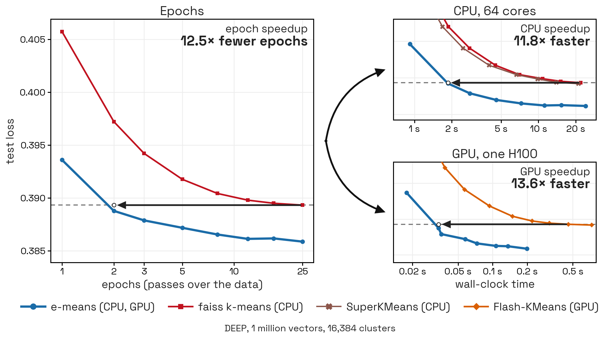
An order of magnitude less epochs

Across a large range of scales and datasets, e-means reaches a test loss below Lloyd's at 25 epochs, in 1.2 to 3 epochs. Measured end to end, that is a 10–45× wall-clock reduction on GPU against the state-of-the-art Lloyd implementation (Flash-KMeans^[2]), and 8–15× on CPU against Faiss^[1]. Speed and quality usually trade against each other in k-means, while e-means achieves both better speed and loss.

The k-means problem

Given a fixed dataset of n points X = {x₁, ..., x_n} ⊂ R^d and an integer k, the k-means problem is to find k centroids C = (c₁, ..., c_k) minimizing the mean squared distance between each point and its nearest centroid:

\[ \mathrm{MSE}(X, C) = \frac{1}{n} \sum_{i=1}^{n} \|x_i - c_{a(i)}\|^2, \qquad a(i) = \arg\min_{j \in \{1,\dots,k\}} \|x_i - c_j\|^2 \]

It's a static dataset, unlike codebook learning inside VQ-VAEs, where the distribution to cluster is constantly moving.

The e-means project

The goal of e-means is to provide a modern optimization rule for the k-means problem. We started this project from the following observations:

• k-means is one of the rare problems in machine learning where full-batch optimization is still widely used.
• Mini-batch k-means methods in the literature exist^[3],[4],[5], but are mostly based on the MacQueen update rule, released in 1967.
• Modern deep learning offers optimization tools that can enhance mini-batch methods.

For e-means, we chose to do mini-batch updates with exponential moving averages^[6], which we found to be most efficient for the k-means problem. Contrary to previous mini-batch approaches, e-means requires no hyperparameter tuning because it automatically sets the batch size and step size with scaling laws (see Automatic hyperparameter tuning with scaling laws). In addition, e-means improves the initialization and the dead-cluster revival strategy, adds a cosine-scheduled decay rate, and introduces a finalization stage that reduces the training loss for a negligible runtime penalty at the end of training. e-means is highly parallelizable, and comes with specialized kernels that translate its algorithmic advantage into wall-clock speedups.

The centroid update rules

The centroid update rule is the central component of e-means. This section aims to provide an overview of update rules for k-means clustering. All methods maintain, for each cluster j, a sum S_j and a count N_j of the points assigned to it, and take the centroid as their ratio:

\[ c_j = S_j / N_j \]

They differ only in how S_j and N_j are updated. Below, s_j and n_j denote the sum and the count of the points in the current batch that are assigned to cluster j (both zero if none are).

Lloyd’s algorithm^[7] assigns every point to its nearest centroid and recomputes the statistics from scratch, using the full dataset as the batch:

\[ S_j \leftarrow s_j, \qquad\quad N_j \leftarrow n_j \]

so c_j is the exact mean of the points currently assigned to it. Each update costs one full pass over the data, and the procedure is repeated a fixed number of times (typically 20 to 50 iterations).

MacQueen’s update^[3] accumulates the statistics without ever discarding them:

\[ S_j \leftarrow S_j + s_j, \qquad\quad N_j \leftarrow N_j + n_j \]

so c_j is the uniform mean of every point assigned to cluster j since the start of training, including points assigned under earlier, possibly poor, centroid positions. This was later partially addressed by Staleness-Reduction Mini-Batch K-Means^[8], a hybrid method between k-means and MacQueen. They obtained important speedups, but only on very low numbers of clusters.

e-means works on mini-batches and replaces this sum with an exponential moving average:

\[ S_j \leftarrow (1-\alpha)\,S_j + \alpha\, s_j, \qquad\quad N_j \leftarrow (1-\alpha)\,N_j + \alpha\, n_j \]

so older assignments are forgotten at rate α, and the centroid tracks recent assignments rather than the whole history. This update rule is typically used for moving distributions, hence their adoption for training VQ-VAEs^[6]. What we found is that it’s also extremely efficient for static datasets if it’s combined with e-means’ other components, and hyperparameters are properly tuned.

Why exponential moving average updates and not gradient descent?

The e-means project started from previous work at Meta FAIR by Hugo Touvron and Hervé Jégou, who had found that mini-batch k-means by gradient descent could beat Lloyd’s algorithm. While I could reproduce these results, I found that the performance of gradient-descent based centroid updates is unstable at large learning rates, unlike exponential moving average updates. I suspect that is because EMA updates guarantee that the centroid is always in the convex hull of points assigned to it, while gradient descent updates may overshoot past that hull.

In order to achieve the lowest loss at a fixed number of epochs, we chose exponential moving average updates, hence the name e-means for our method.

Lloyd is a special case of e-means: hyperparameter study

If you set the batch to the full dataset, B = n, and α = 1, then N_j and S_j become exactly the count and sum of the whole cluster, so one e-means iteration becomes exactly one Lloyd iteration. Lloyd is an extreme case of e-means without cosine scheduling on the learning rate. However, our hyperparameter search found that this extreme setting is highly suboptimal, which explains why e-means largely outperforms Lloyd. Below, the loss is measured for every batch size B and step α: Lloyd lands in a corner, well outside the region where the loss is lowest.

This hyperparameter study motivated us to derive scaling laws that automatically pick the optimal batch size B and step size α.

e-means better escapes local minima

To better understand why e-means reaches better losses than Lloyd at convergence, we plotted a few trainings on toy datasets to evaluate their ability to escape local minima. Repeating trainings over 200 seeds, we found that e-means is much less likely to fall in pathological configurations compared to Lloyd.

Our explanation for that is that mini-batches provide more noisy updates that are more likely to explore the optimization landscape and escape local minima. Lloyd, with its always decreasing loss, is more likely to exploit found local minima and never escape them.

Automatic hyperparameter tuning with scaling laws

An essential property of e-means is that practitioners don't need to set any additional hyperparameter compared to Lloyd's algorithm. We fitted two scaling laws to set the batch size B and step size α₀ from any problem's characteristics (n, k, T), and found them to exhibit strong generalization on unseen datasets and problem scales.

\[ B = c_B \, k^{b_k} \, n^{b_n} \, T^{b_T} \]

\[ \alpha_0 = \min\!\Big(c_\alpha \, k^{a_k} \, B^{a_B} \, n^{a_n} \, T^{a_T},\; 1\Big) \]

We propose two equations to choose the batch, the default law and the quality law. The “quality law” trades off throughput for better clustering quality against the “default” law. Below we plot the training data for our scaling laws: validation MSE against step size α₀ (left) and batch size B (right).

The importance of dead-cluster revival

The main issue with mini-batch k-means is that it is prone to “dead” clusters, centroids that end up with zero assigned points during optimization. This reduces the effective size of the codebook, which is especially problematic for the large codebooks increasingly used today.

A common mitigation is to reinitialize clusters that fall below a certain size threshold, as done in EnCodec^[10], where dead centroids are simply replaced by random samples drawn from the incoming batch. While this helps, it does not fully resolve the issue. Instead of sampling arbitrary points from the batch, we revive dead clusters by splitting large, existing ones: we sample an active cluster with probability proportional to its size and split it into two. We found this approach, adapted from Faiss k-means, to be significantly more effective at eliminating dead clusters and preserving codebook capacity.

Extensive experimental validation

We validated e-means on 24 different embedding and synthetic datasets and configurations (see paper). For the video we ran 234 configurations of e-means against k-means (16 datasets, 100k to 100M points): explore every curve in the results map.

Library and code

from faiss.contrib.e_means import Emeans # NumpyEmeans for NumPy em = Emeans(d, k, nepochs=T) # T epochs (5 by default) centroids, labels = em.train(x) # x: a PyTorch tensor (n, d) # labels: each vector's cluster in the last epoch

Repo: faiss/contrib/e_means.

References

1. M. Douze, A. Guzhva, C. Deng, J. Johnson, G. Szilvasy, P.-E. Mazaré, M. Lomeli, L. Hosseini, H. Jégou. "The Faiss library." arXiv:2401.08281, 2024. ↑
2. S. Yang, H. Xi, Y. Zhao, M. Li, X. Fan, J. Zhang, H. Cai, Y. Lin, X. Li, K. Keutzer, S. Han, C. Xu, I. Stoica. "Flash-KMeans: Fast and Memory-Efficient Exact K-Means." arXiv:2603.09229, 2026. ↑
3. J. MacQueen. "Some Methods for Classification and Analysis of Multivariate Observations." Proceedings of the Fifth Berkeley Symposium on Mathematical Statistics and Probability, 1:281–297, 1967. ↑
4. D. Sculley. "Web-Scale K-Means Clustering." WWW, 2010. ↑
5. J. Newling, F. Fleuret. "Nested Mini-Batch K-Means." NeurIPS, 2016. ↑
6. A. van den Oord, O. Vinyals, K. Kavukcuoglu. "Neural Discrete Representation Learning." NeurIPS, 2017. ↑
7. S. Lloyd. "Least squares quantization in PCM." IEEE Transactions on Information Theory, 28(2):129–137, 1982 (circulated as a Bell Labs technical note since 1957). ↑
8. X. Zhu, J. Sun, Z. He, J. Jiang, Z. Wang. "Staleness-Reduction Mini-Batch K-Means." IEEE Transactions on Neural Networks and Learning Systems, 35(10):14424–14436, 2024. ↑
9. E. Jääsaari, V. Hyvönen, M. Ceccarello, T. Roos, M. Aumüller. "VIBE: Vector Index Benchmark for Embeddings." arXiv:2505.17810, 2025. ↑
10. A. Défossez, J. Copet, G. Synnaeve, Y. Adi. "High Fidelity Neural Audio Compression." Transactions on Machine Learning Research, 2023. arXiv:2210.13438. ↑