“One Guinness, please!” says a customer to a barkeep, who flips a branded pint glass and catches it under the tap. The barkeep begins a multistep pour process lasting precisely 119.5 seconds, which, whether it’s a marketing gimmick or a marvel of alcoholic engineering, has become a beloved ritual in Irish pubs worldwide. The result: a rich stout with a perfect froth layer like an earthy milkshake.

The Guinness brewery has been known for innovative methods ever since founder Arthur Guinness signed a 9,000-year lease in Dublin for £45 a year. For example, a mathematician-turned-brewer invented a chemical technique there after four years of tinkering that gives the brewery’s namesake stout its velvety head. The method, which involves adding nitrogen gas to kegs and to little balls inside cans of Guinness, led to today’s hugely popular “nitro” brews for beer and coffee.

But the most influential innovation to come out of the brewery by far has nothing to do with beer. It was the birthplace of the t-test, one of the most important statistical techniques in all of science. When scientists declare their findings “statistically significant,” they very often use a t-test to make that determination. How does this work, and why did it originate in beer brewing, of all places?

If you're enjoying this article, consider supporting our award-winning journalism by subscribing. By purchasing a subscription you are helping to ensure the future of impactful stories about the discoveries and ideas shaping our world today.

Near the start of the 20th century, Guinness had been in operation for almost 150 years and towered over its competitors as the world’s largest brewery. Until then, quality control on its products consisted of rough eyeballing and smell tests. But the demands of global expansion motivated Guinness leaders to revamp their approach to target consistency and industrial-grade rigor. The company hired a team of brainiacs and gave them latitude to pursue research questions in service of the perfect brew. The brewery became a hub of experimentation to answer an array of questions: Where do the best barley varieties grow? What is the ideal saccharine level in malt extract? How much did the latest ad campaign increase sales?

Amid the flurry of scientific energy, the team faced a persistent problem: interpreting its data in the face of small sample sizes. One challenge the brewers confronted involves hop flowers, essential ingredients in Guinness that impart a bitter flavor and act as a natural preservative. To assess the quality of hops, brewers measured the soft resin content in the plants. Let’s say they deemed 8 percent a good and typical value. Testing every flower in the crop wasn’t economically viable, however. So they did what any good scientist would do and tested random samples of flowers.

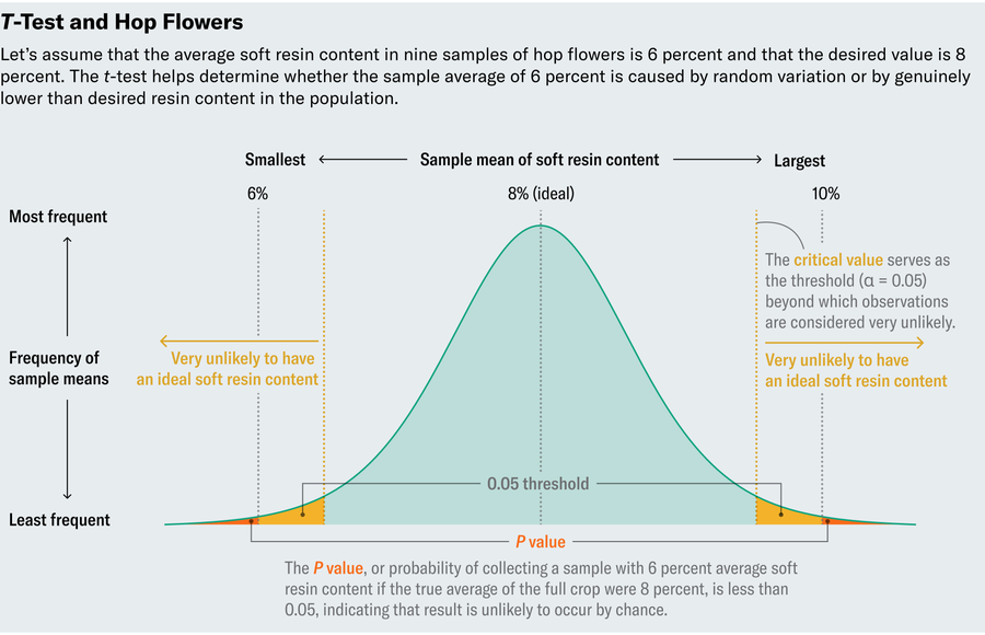
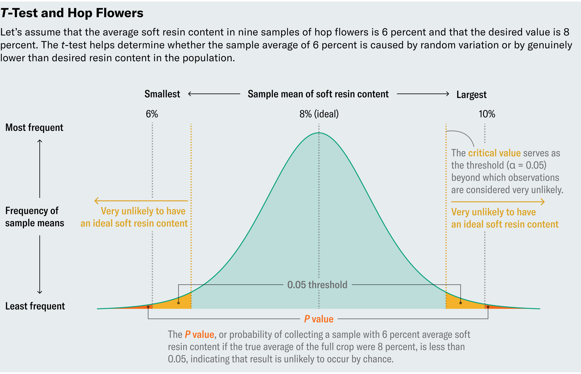
Let’s inspect a made-up example. Suppose we measure soft resin content in nine samples and, because samples vary, observe a range of values from 4 percent to 10 percent, with an average of 6 percent—too low. Does that mean we should dump the crop? Uncertainty creeps in from two possible explanations for the low measurements. Either the crop really does contain unusually low soft resin content, or though the samples contain low levels, the full crop is actually fine. The whole point of taking random samples is to rely on them as faithful representatives of the full crop, but perhaps we were unlucky by choosing samples with uncharacteristically low levels. (We only tested nine, after all.) In other words, should we consider the low levels in our samples significantly different from 8 percent or mere natural variation?

This quandary is not unique to brewing. Rather, it pervades all scientific inquiry. Suppose that in a medical trial, both the treatment group and placebo group improve, but the treatment group fares a little better. Does that provide sufficient grounds to recommend the medication? What if I told you that both groups actually received two different placebos? Would you be tempted to conclude that the placebo in the group with better outcomes must have medicinal properties? Or could it be that when you track a group of people, some of them will just naturally improve, sometimes by a little and sometimes by a lot? Again, this boils down to a question of statistical significance.

The theory underlying these perennial questions in the domain of small sample sizes hadn’t been developed until Guinness came on the scene—specifically, not until William Sealy Gosset, head experimental brewer at Guinness in the early 20th century, invented the t-test. The concept of statistical significance predated Gosset, but prior statisticians worked in the regime of large sample sizes. To appreciate why this distinction matters, we need to understand how one would determine statistical significance.

Remember, the hops samples in our scenario have an average soft resin content of 6 percent, and we want to know whether the average in the full crop actually differs from the desired 8 percent or if we just got unlucky with our sample. So we’ll ask the question: What is the probability that we would observe such an extreme value (6 percent) if the full crop was in fact typical (with an average of 8 percent)?Traditionally, if this probability, called a P value, lies below 0.05, then we deem the deviation statistically significant, although different applications call for different thresholds.

Often two separate factors affect the P value: how far a sample deviates from what is expected in a population and how common big deviations are. Think of this as a tug-of-war between signal and noise. The difference between our observed mean (6 percent) and our desired one (8 percent) provides the signal—the larger this difference, the more likely the crop really does have low soft resin content. The standard deviation among flowers brings the noise. Standard deviation measures how spread out the data are around the mean; small values indicate that the data hover near the mean, and larger values imply wider variation. If the soft resin content typically fluctuates widely across buds (in other words, has a high standard deviation), then maybe the 6 percent average in our sample shouldn’t concern us. But if flowers tend to exhibit consistency (or a low standard deviation), then 6 percent may indicate a true deviation from the desired 8 percent.

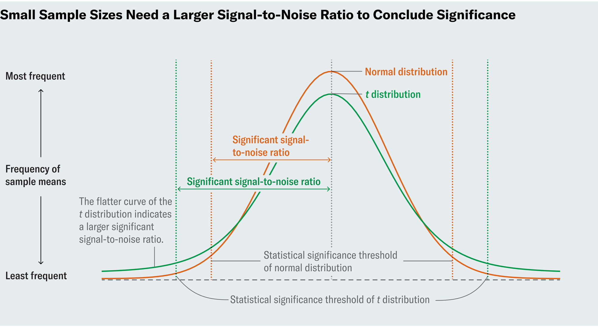
To determine a P value in an ideal world, we’d start by calculating the signal-to-noise ratio. The higher this ratio, the more confidence we have in the significance of our findings because a high ratio indicates that we’ve found a true deviation. But what counts as high signal-to-noise? To deem 6 percent significantly different from 8 percent, we specifically want to know when the signal-to-noise ratio is so high that it only has a 5 percent chance of occurring in a world where an 8 percent resin content is the norm. Statisticians in Gosset’s time knew that if you were to run an experiment many times, calculate the signal-to-noise ratio in each of those experiments and graph the results, that plot would resemble a “standard normal distribution”—the familiar bell curve. Because the normal distribution is well understood and documented, you can look up in a table how large the ratio must be to reach the 5 percent threshold (or any other threshold).

Gosset recognized that this approach only worked with large sample sizes, whereas small samples of hops wouldn’t guarantee that normal distribution. So he meticulously tabulated new distributions for smaller sample sizes. Now known as t-distributions, these plots resemble the normal distribution in that they’re bell-shaped, but the curves of the bell don’t drop off as sharply. That translates to needing an even larger signal-to-noise ratio to conclude significance. His t-test allows us to make inferences in settings where we couldn’t before.

Mathematical consultant John D. Cook mused on his blog in 2008 that perhaps it should not surprise us that the t-test originated at a brewery as opposed to, say, a winery. Brewers demand consistency in their product, whereas vintners revel in variety. Wines have “good years,” and each bottle tells a story, but you want every pour of Guinness to deliver the same trademark taste. In this case, uniformity inspired innovation.

Gosset solved many problems at the brewery with his new technique. The self-taught statistician published his t-test under the pseudonym “Student” because Guinness didn’t want to tip off competitors to its research. Although Gosset pioneered industrial quality control and contributed loads of other ideas to quantitative research, most textbooks still call his great achievement the “Student’s t-test.” History may have neglected his name, but he could be proud that the t-test is one of the most widely used statistical tools in science to this day. Perhaps his accomplishment belongs in Guinness World Records (the idea for which was dreamed up by Guinness’s managing director in the 1950s). Cheers to that.