What do Radamacher Complexity and mean field approximations have to do with kin and group selection models in evolutionary biology? And what might consideration of the Radamacher Complexity of kin and group selection models suggest to us about cooperation and competition in human groups? Here are tentative answers to what seem like important questions that nobody is asking.

Group Selection in Evolutionary Biology

The Puzzle of Altruism

Curious students learning the theory of natural selection for the first time have been known to ask: "What about altruism?" What explains how animals, and especially humans, sometimes make a willing sacrifice of their own self-interest for others? Charles Darwin himself acknowledged in the Origin of Species that this is a "special difficulty, which at first appeared ... insuperable, and actually fatal to my whole theory." Darwin's own answer, using neuter or sterile female insects (like worker ants or bees) as an example, was as follows:

We can see how useful their production may have been to a social community of insects, on the same principle that the division of labour is useful to civilised man. As ants work by inherited instincts and by inherited tools or weapons, and not by acquired knowledge and manufactured instruments, a perfect division of labour could be effected with them only by the workers being sterile; for had they been fertile, they would have intercrossed, and their instincts and structure would have become blended. And nature has, as I believe, effected this admirable division of labour in the communities of ants, by the means of natural selection. But I am bound to confess, that, with all my faith in this principle, I should never have anticipated that natural selection could have been efficient in so high a degree, had not the case of these neuter insects convinced me of the fact.

Origin of the Species, Chapter VII (last paragraph before Summary) (1859).

The Kin Selection Theory Solution

Darwin's emphasis on "inherited instincts" vs. "acquired knowledge", which enforced "a perfect division of labour" (my italics) that "could be effected ... only by the workers being sterile" was in 1964 formalized by William D. Hamilton into a mathematical rule:

$$rB > C$$

Where:

r represents the genetic relatedness of the recipient of an altruistic act to the actor
B represents the benefit gained by the recipient of the altruistic act
C represents the reproductive cost to the actor of performing the act

The Wikipedia article on kin selection provides a representative sample of the success that Hamilton's Rule has had in its simplicity and predictive power. Before Hamilton's Rule, Darwin's theory of natural selection lacked precision in making predictions about when pro-social behavior by individuals. Hamilton's Rule and later elaborations of kin selection theory — especially those ramifying on the implications of a default to reciprocity in repeated social interactions — have been successful at explaining many observations of altruism that might otherwise be puzzling.

The Group Selection Theory Alternative

Notwithstanding the success of Hamilton Rule's, Nowak, Tarnita, and Wilson (hereinafter, NTW) published in 2010 The evolution of eusociality, a manifesto arguing that kin selection and inclusive fitness theory in evolutionary biology are "not a general theory of evolution," and that Hamilton's Rule specifically "almost never holds." According to NTW, "inclusive fitness considerations rest on fragile assumptions, which do not hold in general."

What assumptions? In their own words: "Inclusive fitness theory claims to be a gene-centered approach, but instead it is ‘worker-centered’. It puts the worker into the center of the analysis...", an approach that requires tracking the effects of an action on relatives, a detailed accounting that is so complex that it must adopt simplifying assumptions (such as pairwise additive interactions or weak selection) to be tractable.

NTW proposed an alternative a model (detailed in Box 1 and Supplementary Information Part C) that shifted the focus from the individual worker's decisions to the overall reprodutive success of the queen and colony. An important claim in this essay is that group selection theory as presented in NTW 2010 represents a mean-field theory as that term is used in theoretical physics to describe condensed matter and quantum fields.

In the next section, I'll explain what a mean field theory is and how the mathematical model of NTW 2010 can be understood as a mean field theory. At the end of that section, I'll explain how this recognition helps resolve much of the controversy among evolutionary biologists over whether kin selection theory or group selection theory are correct.

Group Selection Theory as a Mean Field Approximation

Mean Field Theories in Physics

Physicists have been faced with the same mathematical difficulty in tracking the larger scale and longer term effects of a single particle's action on its neighbors (the "worker-centered" approach necessitated by kin selection theory) for over 100 years. Especially before the invention of computers, the ability to do mathematical analysis of the cumulative effects of interactions among many particles was basically impossible as a practical matter. This is why as early as 1907, Pierre Curie and Pierre Weiss proposed that instead of tracking all interactions between the many particles in a material, that an approximation of those interactions be made by assuming an averaged over or effective interaction — a "mean field theory."

Even after the invention of computers, mean field theories have been useful to physicists. Only in the case of weak interactions is it possible to do numerical approximations of the behavior of systems with even a tiny fraction of the number of molecules in a real system — by Avogadro's number (≈\(10^{23}\)) a glass contains a trillion trillion molecules. Even the number of water molecules that have dissociated into ions at pH 7 and standard temperature and pressure is 10s of thousands of trillions! Even with computers, modeling the interactions of each molecule with all other molecules in the glass is impossible unless you assume that the glass is almost empty — that is, that the water molecules are in the gas phase and only occasionally bumping into each other.

But much of behavior that's interesting to somebody studying how molecules (or electrons, or whatever) interact is the behavior that obtains when they're strongly interacting. For studying strong interactions of trillions of anything, you need to make approximations, and mean field theories represent one set of approximations.

NTW 2010 Present a Mean Field Theory

NTW 2010 approximate by averaging over the worker contributions across the colony. Referring to Part C of the Supplementary Information, the complex social interactions within the colony — foraging, defense, nursing, and potential conflicts — are not tracked individually. Instead, they are abstracted into averaged demographic parameters. The model defines the queen's reproductive rate (\(b_i\)) and death rate (\(d_i\)) as functions of the colony size \(i\). The specific contribution of any single worker is ignored; what matters is the net effect of having \(i-1\) workers on the queen’s fitness. This replacement of detailed, localized interactions with an averaged effect based on colony size is a mean field approximation.

NTW 2010 ignore what in physics would be called localized correlations and in Hamilton's Rule is called "relatedness" (\(r\)). Under their mean field theory, the success of an individual allele is based on the demographic advantages conferred on the queen, regardless of the details of relatedness. NTW explicitly acknowledge this:

In our model relatedness does not drive the evolution of eusociality. ... The competition between the eusocial and the solitary allele is described by a standard selection equation.

Box 1.

The omission of the detailed local correlations (here, the genetic relatedness of workers to the queen) that are central to kin selection theory here is a characteristic of all mean field theories. The group selection theory proposed in NTW 2010 achieves its simplifications by viewing the workers not as independent agents making strategic decisions or engaging in a cooperative dilemma, but instead as extensions of the queen:

[T]he workers are not independent agents. Their properties depend on the genotype of the queen and the sperm she has stored. Their properties are determined by the alleles that are present in the queen (both in her own genome and in that of the sperm she has stored). The workers can be seen as ‘robots’ that are built by the queen. They are part of the queen’s strategy for reproduction.

Supplementary Information at 38.

By treating workers as "robots" rather than independent evolutionary actors, the model explicitly glosses over the microscopic strategic interactions and behavioral fluctuations within the colony, focusing only on the macroscopic output of the colony as a whole.

Reconciling Kin and Group Selection Theory as Valid Alternative Models

If you've been following along, then at this point you probably have a sense that there's a mathematical way to resolve the arguments among evolutionary biologists over whether kin or group selection theory is the one true theory of evolution by natural selection. The mathematical answer is that they're both valid models of natural selection. While kin selection theory may ultimately be the most rigorous method for expressing the process of genetic evolution, it is often intractable as a model of how an actual colony of ants or bees — much less humans — behave in nature. In many cases, a mean field approximation like the one proposed in NTW 2010 provides a useful model of how the colony behaves by averaging over the details of individual workers.

Bearing that in mind, it's an interesting exercise to review the critique of group selection theory offered by Steven Pinker and responses here, and I was not able to overcome the tempatation to review the arguments presented here in view of this mathematical perspective.

I love Steven Pinker, who I consider to be a clear thinker that also seems to operate with a high level of tolerance and integrity. But Pinker, Dawkins, Coyne and others (whom I also admire) are as bad as Nowak, Tarnitas, and Wilson (both E.O. and David Sloan) in their refusal to acknowledge any merit in an alternative model. Ironically, it is in his unselfconscious teasing of physicists who "assume a spherical cow" (in order to help a farmer increase milk yields), that Pinker reveals the ultimate weakness of his position — a failure to acknowledge the pragmatic value that an approximation might have for understanding a phenomena that is otherwise too complex to be modeled at all. I will grant the group of Pinker, Dawkins, and Coyne at least an honorable mention for acknowledging that the two theories can produce the same predictions under the right assumptions, but I'm disappointed at their refusal to acknowledge the potential instrumental value of mean field approximations in describing collective behavior — why should we not explore and use any mathematical model that offers us a mathematical model of aspects of natural selection that would otherise be intractable? Indeed, one has the sense that the debate is less about the merits of one mathematical model vs. another than it is about fascism vs. individualism or communism vs. democracy or some other (in some cases, thinly) suppressed premise.

Among those who participated, Joseph Henrich and David Queller seem to come closest to getting it right. Henrich emphasizes that group selection theory is simply a model that has proved useful in certain regimes. ("Which accounting system is best entirely depends on the problem and the assumptions one is willing to make in obtaining an answer.") Queller uses a "two languages" metaphor, acknowledging that the two models are "mathematically equivalent" frameworks that "divide up fitness in slightly different ways," recognizing that both can be valid and useful. But nobody explicitly identifies group selection theory as a mean field approximation of kin selection theory.

Radamacher Complexity as Measure of Model Richness

Having sketched out a reconcilation of what otherwise might seem like conflicting models of evolution, I turn now to showing how a metric developed in machine learning theory, Radamacher Complexity, can be used to provide a mathematical measure of the instrumental value of one model vs. the other.

The Example of Non-Additive Games

For definiteness and ease of explanation, let's take a regime explicitly addressed in NTW 2010, Section 7.2. This is the regime in which the fitness effect of actions combines non-linearly. In an additive game, the total fitness payoff for a worker is simply the sum of individual contributions by each worker and her partners. If cooperation provides a benefit B at cost C to a particular worker, these benefits and costs are constant regardless of what other workers do. In a non-additive game, by contrast, there is an additional effect that arises when certain workers act together, so that the benefit B may be achieved only upon some threshold of cooperation among the workers.

From 3-Person Stag Hunt to Ant and Bee Colonies

The 3-person stag hunt game described by NTW 2010 in Section 7.2 demonstrates non-additive interactions where a group (of 3 stag hunters) can only accomplish a task (the successful hunt) if all three members cooperate. If all three cooperate, each pays cost c but receives benefit b (payoff: b-c for each). However, if only one or two members cooperate, the hunt fails and cooperators pay the cost without any benefit (payoffs: -c for cooperators, 0 for defectors), making the benefits synergistic rather than simply additive from pairwise interactions.

A kin selection model of three 3-worker groups built up from n members is still tractable small n. But in most more realistic models of workers in an ant or bee colony, kin selection models become intractable. Consider extending the 3-person stag hunt example from Section 7.2 as follows to polyandrous colonies evolving with environmental shocks:

class SynergisticColonyModel:
    def __init__(self, max_caste_types=5, max_colony_size=1000):
        # Fitness depends on synchronized caste combinations
        # e.g., foragers + nurses + guards in specific ratios
        self.caste_interactions = self.generate_synergistic_matrix()
    
    def fitness(self, colony_composition):
        # Non-additive: certain combinations produce emergent benefits
        # Intractable because we need to evaluate all possible 
        # combinations of related individuals across castes
        return self.evaluate_higher_order_interactions(colony_composition)

If we let the population evolve with:

• \(N_{spatial}\) = 100 (patches in environment)
• \(N_{colony}\) ∈ [1, 1000] (individuals per colony)
• \(G\) = 10 (relevant genetic loci)
• \(P\) = 5 (pathogen strains)

To calculate inclusive fitness directly, we'd need to track:

1. Relatedness between all pairs: O(N_colony²) per colony
2. How relatedness changes with colony composition: O(2^G) possible genetic states
3. Spatial correlations in relatedness: O(N_spatial²) comparisons
4. Pathogen-mediated selection on genetic diversity: O(P × 2^G) interactions

Thus the total calculations required per generation would be of order:

$$O(N_{spatial} × N_{colony}^2 × 2^G × P) ≈ 100 × 10^6 × 1024 × 5 ≈ 5 × 10^{11}$$

A Kin Theory Based Neural Network Approximation

Let's say that we're ideologically pre-committed to kin selection theory, and are therefore unwilling on principle to consider making a mean field approximation. It's 2025 and Nvidia now has attained a market cap of $5 trillion selling GPUs optimized to do machine learning! Instead of tracking all these states explicitly, we can train a neural network with a compressed representation:

def neural_approximation(colony_state, spatial_context):
    # Reduce N_colony × G dimensional genetic info to fixed embedding
    genetic_embedding = embed_relatedness_pattern(colony_state)  # O(1) output size
    
    # Reduce N_spatial dimensional context to fixed size
    spatial_embedding = embed_spatial_structure(spatial_context)  # O(1) output size
    
    # Predict fitness with fixed complexity
    return fitness_network(genetic_embedding, spatial_embedding)  # O(1) computation

This is still an approximation, of course, but as basically everybody understands today, given enough data, neural networks can be surprisingly successful at capturing relatively nuanced features of large, complex data sets. This is not the only approach that might be taken to building a realistic kin selection model of natural selection of an actual ant or bee colony, of course. But I believe it's at least representative of what might be considered state of the art.

The Group Selection (Mean Field) Approximation Alternative

Now let's say tht we're ideologically pre-committed to group selection theory, and must therefore insist on using a mean field approximation to model natural selection in the same ant or bee colony. Following NTW 2010's approach:

def group_selection_mean_field(params):
    # Aggregate at colony level
    avg_colony_resistance = f(genetic_diversity)
    colony_productivity = g(queen_mating_number, worker_number)
    
    # Simple ODEs as in NTW Part C
    dx_mono/dt = (b_mono * resistance_mono - d_mono) * x_mono
    dx_poly/dt = (b_poly * resistance_poly - d_poly) * x_poly
    
    return equilibrium_frequencies

And now we have an alternative (tractable) mathematical model of natural selection. Both models are now tractable to computation on large clusters. So which of these models is more useful? At this point, we could fall back to debates about collectivism vs. individualism, the Scottish Enlightenment vs. Confucianism, etc. But the second important claim in this essay is that the machine learning concept of Radamacher Complexity gives us a mathematical way to measure and choose between these models.

Radamacher Complexity Comparison

What is Radamacher Complexity?

Radamacher Complexity boils down to a measure of how easy (or difficult) a theory is to falsify with (out of training sample) experimental evidence. To calculate Radamacher Complexity, you start with the predictions your model would make for a given set of measurements, then randomly flip the predictions and check whether the model would still fit the predictions. Models with high Radamacher Complexity have the potential to be more accurate, but are also more likely to overfit whatever data was used to build the model. Models with lower Radamacher Complexity that give good predictions are more robust in the sense that they have higher predictive power given a fixed amount of data used for training. Lower Radamacher Complexity is, therefore, stricly better so long as model predictions are accurate.

A simple example of machine learning models trained to detect whether an email is spam or not might help illustrate what Radamacher Complexity is and how it is calculated:

The Setup: Spam Detection

Imagine we are building a model to classify emails as Spam (+1) or Not Spam (-1).

• The Data (\(m\)): We have a tiny dataset of \(m=4\) emails.

  • Email 1 (\(x_1\)): "Cheap meds now" (Actual: Spam +1)
  • Email 2 (\(x_2\)): "Meeting at 3 PM" (Actual: Not Spam -1)
  • Email 3 (\(x_3\)): "Win a free cruise" (Actual: Spam +1)
  • Email 4 (\(x_4\)): "Project status update" (Actual: Not Spam -1)

• \(m\) (Dimension of the vectors): This is purely the size of your dataset.

  • Here, \(m = 4\). Every vector \(a\) in our set \(A\) will have 4 entries, corresponding to the 4 emails above.

• \(n\) (Number of vectors in set \(A\)): This is the number of different ways your model can make specific mistakes.

  • Even though a model has infinite possible weights, it can only classify these 4 emails in a finite number of ways (specifically, \(2^4 = 16\) possible combinations of labels).
  • \(n\) is how many of those 16 combinations your model is actually capable of producing.

Model Predictions: (\(a\))

To make the intuition easiest, let's slightly adjust the definition of the vector \(a\) to be the model's raw predictions rather than losses. (The math is equivalent, but "fitting noise" is easier to see this way).

• Let vector \(a = [h(x_1), h(x_2), h(x_3), h(x_4)]\), where \(h(x_i)\) is the model's prediction (-1 or +1) for email \(i\).
• A perfect model for our data would produce the vector: [+1, -1, +1, -1].

Computing Radamacher Complexity: Fitting Noise

To find the Rademacher Complexity, we don't use the real labels. We use Rademacher noise (\(\sigma\)) as the labels.

We generate a random \(\sigma\) vector, say: [+1, +1, -1, +1].

• This is "noise" because we are essentially lying to the model. We are telling it:
  • "Cheap meds" is Spam (+1)
  • "Meeting at 3 PM" is Spam (+1) (Lie)
  • "Win a free cruise" is Not Spam (-1) (Lie)
  • "Project status update" is Spam (+1) (Lie)

We then train our two models to see if they can learn these "crazy" labels.

Model A: The Linear Model (Low Complexity)

A linear model tries to separate these emails with a straight line based on features (e.g., count of the word "free").

• Challenge: Can a straight line classify "Meeting" and "Project update" as opposites, while also classifying "Meds" and "Cruise" as opposites?
• Reality: Probably not. If it learns "free" indicates non-spam (to fit the lie about Email 3), it will likely misclassify Email 1.
• Result: The linear model cannot produce a prediction vector \(a\) that matches this noise \(\sigma\). The best it might do is get 2 out of 4 right.
• Correlation: The sum \(\sum \sigma_i a_i\) will be low (e.g., \(1+1-1-1 = 0\)).

Model B: Deep Neural Network (High Complexity)

A deep neural net has millions of parameters. It doesn't just look at "free"; it looks at every character combination.

• Challenge: Can it learn the crazy labels?
• Reality: Yes. It can likely find a very specific, convoluted set of weights that perfectly memorizes this specific noise pattern.
• Result: The neural net can produce a prediction vector \(a\) that exactly matches \(\sigma\): [+1, +1, -1, +1].
• Correlation: The sum \(\sum \sigma_i a_i\) will be maximum (\(1+1+1+1 = 4\)).

The Spam Detection Models Compared

If you repeat this 10,000 times with different random \(\sigma\) noise vectors:

• The Linear Model will rarely be able to match the noise. Its average maximum correlation (and thus its Rademacher Complexity) will be low.
• The Neural Net will almost always be able to perfectly match the noise. Its average maximum correlation will be very high (close to 1.0 on a normalized scale).

Why not try a Radamacher Complexity comparison of group and kin selection models?

The Comparison of Group and Kin Selection Models

If you've followed along this far, then hopefully you already have a sense of how the calculation of Radamacher Complexity might provide a useful metric for comparison of group and kin selection models of natural selection — Radamacher Complexity tells us whether whatever massive dimensionality reduction we've made preserves the essential evolutionary dynamics or loses critical information.

def compare_model_complexity(evolutionary_data, n_epochs=100):
    # Split data into training and test
    train_data, test_data = split_colony_evolution_data(evolutionary_data)
    
    # Compute empirical Rademacher complexities
    R_kin = compute_rademacher_neural(
        train_data,
        model=KinSelectionNN(),
        n_rademacher_samples=1000
    )
    
    R_group = compute_rademacher_meanfield(
        train_data,
        param_bounds=get_biological_bounds(),
        n_rademacher_samples=1000
    )
    
    # Key insight: R_kin >> R_group, but does it help?
    generalization_gap_kin = train_error_kin - test_error_kin
    generalization_gap_group = train_error_group - test_error_group
    
    # The instructive finding would be if:
    # R_kin/R_group ≈ 10-100 (much higher complexity)
    # But if generalization_gap_kin ≈ generalization_gap_group
    # then the added complexity doesn't improve prediction

Why the Comparison is Useful

Finally, we get to the conclusion: estimating the Radamacher Complexity of kin and group selection models provides a (non-ideological!) metric for the relative accuracy of the models. In principle, we can even map out where each approach works:

• Small colonies (N < 50): Both tractable, direct calculation possible
• Medium colonies (50 < N < 500): Neural approximation valuable
• Large colonies (N > 500): Mean field becomes necessary

As an added bonus, an estimation of Radamacher Complexity also gives us a method for testing one NTW 2010's core claims that "relatedness is a consequence of eusociality, but not a cause" through interventional studies and temporal analysis. To be clear, Rademacher Complexity analysis alone cannot validate this claim because multiple causal structures can generate identical observable distributions, but their claim about causality does imply a specific temporal ordering:

class TemporalCausalityTest:
    def test_granger_causality(self, time_series_data):
        # Extract time series
        group_benefits_t = data['ecological_benefits_of_grouping']
        relatedness_t = data['average_within_colony_relatedness']
        eusociality_t = data['degree_of_reproductive_skew']
        
        # NTW predicts this temporal structure:
        # group_benefits[t] → eusociality[t+1] → relatedness[t+2]
        
        # Kin selection predicts:
        # relatedness[t] → eusociality[t+1] → group_benefits[t+2]
        
        # Use Rademacher complexity to compare models with different lag structures
        R_ntw = self.compute_rademacher_temporal(
            model=lambda t: f(group_benefits[t-2], eusociality[t-1]),
            target=relatedness_t
        )
        
        R_kin = self.compute_rademacher_temporal(
            model=lambda t: f(relatedness[t-2], eusociality[t-1]),
            target=group_benefits_t
        )
        
        return R_ntw < R_kin  # Lower complexity suggests correct causal orderW

If the group selection model were to show lower complexity, then that would at least suggest that NTW's causality claim is correct.

A Rough Test of Temporal Causal Models

I went ahead and implemented a rough test of this. You can find the code under an MIT license on GitHub here.

Here are the results:

============================================================
Testing Rademacher Complexity of Temporal Causal Models
Comparing Kin Selection vs Group Selection
============================================================

1. Running complexity comparison experiments...

=== Summary Statistics ===
                           rademacher_complexity         test_error         n_parameters
                                            mean     std       mean     std         mean
true_model test_model                                                                   
group      group_selection                0.0092  0.0007     0.0103  0.0001         90.0
           kin_selection                  0.0144  0.0007     0.0103  0.0001       7350.0
kin        group_selection                0.0161  0.0003     0.0094  0.0001         90.0
           kin_selection                  0.0142  0.0015     0.0094  0.0001       7350.0

True model: group
  Kin selection - Error: 0.0103, Complexity: 0.0144
  Group selection - Error: 0.0103, Complexity: 0.0092
  ✓ Simpler group model generalizes as well with lower complexity

True model: kin
  Kin selection - Error: 0.0094, Complexity: 0.0142
  Group selection - Error: 0.0094, Complexity: 0.0161
  ✗ Complex kin model shows advantage

2. Testing temporal causality (NTW's claim) with enhanced parameters...
This may take a few minutes due to increased sample sizes...

=== Enhanced Temporal Causality Test ===
Testing whether wrong causal direction increases model complexity

Enhanced features:
  - 8 causal factors with different time scales
  - 5 hidden states with decay rates 0.85 to 0.99
  - 15 confounders (autocorrelated, periodic, trending)
  - 3000 time points for better statistical power
  - 5 regularization values tested
  - 1000 Rademacher samples

Complexity measurements (best regularization):
  Correct (causes→effect):      0.0040 (α=10.0)
  Wrong (consequence→effect):   0.0024 (α=10.0)
  Ratio (wrong/correct):        0.61

Predictive error:
  Correct direction:            0.0107
  Wrong direction:              0.0110
  Error ratio (wrong/correct):  1.04

Combined difficulty ratio:      0.82

✗ Result does not clearly support NTW's claim
  The consequence may still contain sufficient information

3. Generating visualizations...

============================================================
CONCLUSIONS
============================================================
1. GROUP SELECTION SUFFICIENT: Simple group model generalizes
   as well as complex kin model for group selection dynamics
3. EFFICIENCY: Group selection is 0.0x more
   parameter-efficient than kin selection

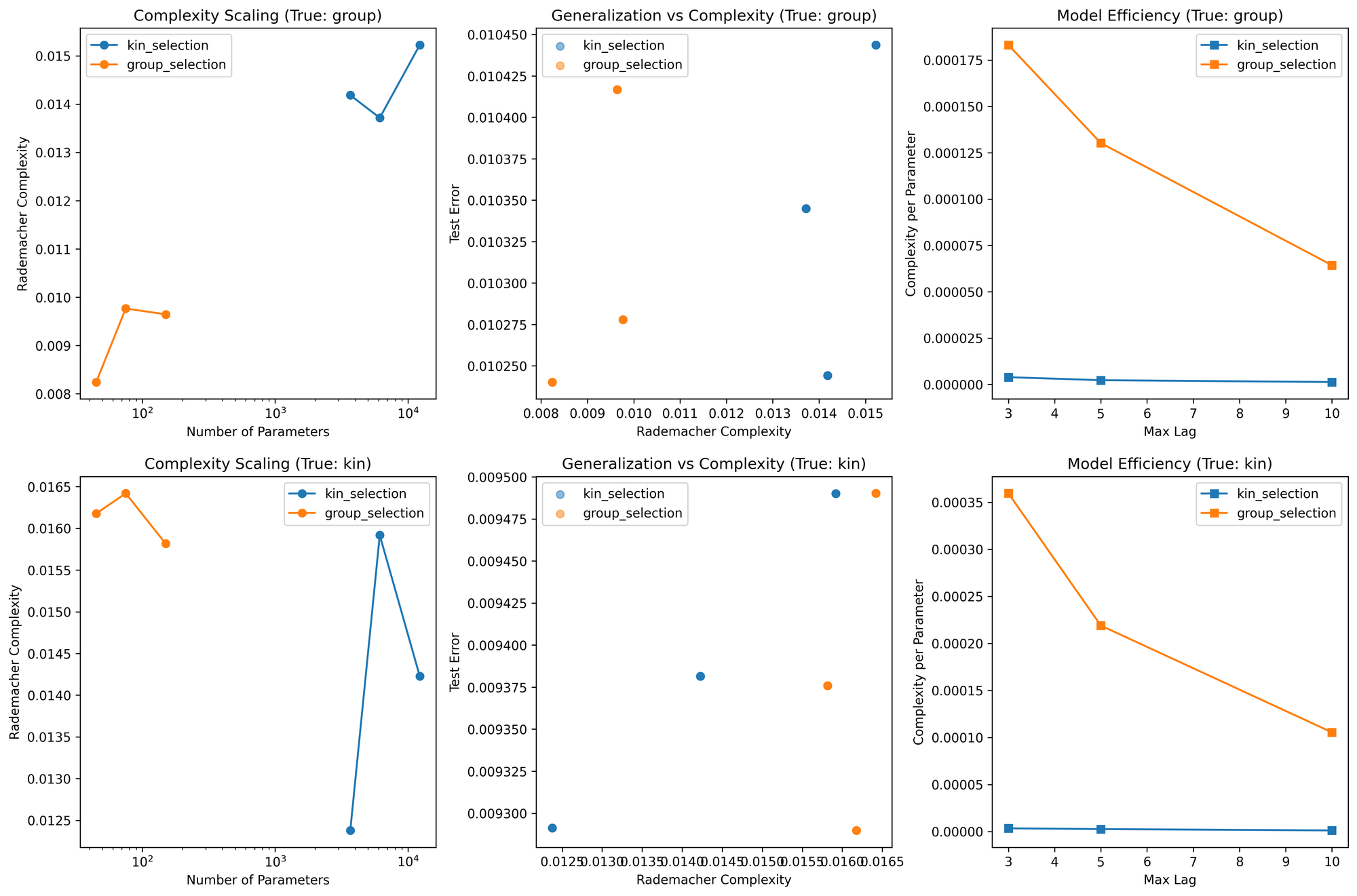
No real surprises. Model results are context dependent. When the "true" dynamics are group selection, both achieve identical test error (0.0103). When the true dynamics are kin selection, both models achieve identical test error (0.0094).

But the Rademacher Complexity reveals some important differences. When modeling group selection dynamics, the group selection model has lower Rademacher Complexity (0.0092) than the kin selection model (0.0144). Conversely, when modeling kin selection dynamics, the group selection model has higher complexity (0.0161) than the kin selection model (0.0142). The group selection model has to work harder to capture kin selection dynamics. It's not always the simpler model.

Perhaps most importantly, the causality test fails to support NTW's claim about causality. The causal chain tested is ecological benefits => eusociality => increased relatedness. Model complexity for the correct causal direction (causes => effect) has Rademacher Complexity 0.0040, while the counter-factual direction (consequence => effect) has lower complexity at 0.0024. Because the complexity is lower for the counter-factual (ratio of 0.61), this test does not validate NTW 2010's claim that "relatedness is a consequence of eusociality, but not a cause."

It is important to emphasize, however, that this test's failure to validate their claim also does not disprove their claim. This is a computational test of temporal causality using Rademacher complexity on synthetic data with specific assumptions. But it is provocative to the extent that it shows the opposite of what NTW might have predicted - the "wrong" causal direction appears less complex to model.

In the final section of this essay, I offer speculative obseverations about what the relationship between group and kin selection models as framed by Radamacher Complexity might imply about the nature of competition among human groups.

Competition as Cooperation

What the mathematical models together seem to be showing is something rather profound about the relationship between competition and cooperation: they are not opposing forces but complementary aspects of natural selection. When groups compete for scarce resources, the selective pressure at the group level can overwhelm individual-level incentives for defection, creating conditions where cooperation becomes the dominant strategy within groups.

Inter-Group Competition as a Catalyst for Intra-Group Cooperation

When groups compete for limited resources—whether territory, food sources, or market share—the groups with superior internal coordination gain decisive advantages. This creates a powerful selection pressure for mechanisms that enhance within-group cooperation, even when such cooperation seems costly at the individual level. The framework developed here offers several insights for understanding human social organization and conflict:

1. The Dual Nature of Social Institutions

Social institutions can be understood as solutions to a two-level optimization problem: they must simultaneously (a) manage internal conflicts to maintain group cohesion and (b) organize collective action for inter-group competition. The most successful institutions are those that align individual incentives with group success, effectively converting the competitive instincts of individuals into cooperative advantages for the group.

2. The Role of Cultural Evolution

While genetic evolution operates slowly, cultural evolution can rapidly adjust the parameters that determine cooperation levels. Cultural innovations — from religious beliefs that increase group cohesion to legal systems that punish defectors — can be understood as mechanisms for moving groups into regions of parameter space where cooperation is evolutionarily stable.

3. The Violence Trap and Institutional Development

This framework aligns remarkably well with North, Wallis, and Weingast's (NWW) theory of violence and social orders. Their "double balance" between political and economic power can be understood as an equilibrium in our multi-level selection framework:

• Limited Access Orders emerge when small coalitions (the dominant coalition) cooperate internally to extract rents from the larger population. This represents a local optimum where within-coalition cooperation is maintained by the threat of violence and the distribution of rents.

• Open Access Orders represent a different equilibrium where cooperation extends beyond narrow coalitions to encompass broader segments of society. The transition requires solving a coordination problem: moving from a Nash equilibrium based on violence potential to one based on impersonal rules and competitive markets.

The mathematical framework suggests why this transition is so difficult: it requires simultaneous changes in multiple parameters (institutional capacity, belief systems, economic structures) to move from one basin of attraction to another. The "doorstep conditions" identified by NWW — rule of law for elites, perpetually lived organizations, and consolidated political control of violence — can be understood as the minimum changes needed to make the transition feasible.

4. Scale-Dependent Governance

The Rademacher Complexity analysis suggests that different scales of human organization require fundamentally different governance approaches:

• Small communities can rely on reputation, reciprocity, and social sanctions—mechanisms that map naturally onto kin selection dynamics.

• Large societies require impersonal institutions, formal laws, and abstract principles of justice—corresponding to mean field approximations where individual relationships matter less than aggregate behaviors.

This might explain why attempts to scale up traditional community-based governance often fail, and why large-scale societies that lose institutional capacity often fragment into smaller, kinship-based units.

The Paradox of Competition-Induced Cooperation

Perhaps the deepest insight from this analysis is that competition between groups can be the strongest force for creating cooperation within groups. This apparent paradox — that conflict begets cooperation — helps explain many puzzling features of human society:

• Why do external threats often lead to increased internal cohesion?
• Why do diverse societies sometimes achieve higher levels of cooperation than homogeneous ones when facing common challenges?
• Why do periods of intense inter-group competition often coincide with peaks of cultural and technological innovation?

The answer lies in the multi-level nature of selection. When groups compete, traits that enhance group success are favored even if they impose costs on individuals. This creates evolutionary pressure for mechanisms—biological, cultural, or institutional—that align individual interests with group success.

Tenative Conclusions

The mathematical framework developed here, connecting evolutionary biology with theoretical physics through the lens of model complexity, offers a path toward understanding one of the fundamental tensions in human society: the simultaneous pull toward individual freedom and collective coordination.

One important insight is that kin selection and group selection are not mutually exclusive theories but complementary descriptions, each of which may be more or less useful at different scales and in different parameter regimes. Like quantum mechanics and classical mechanics in physics, both are correct within their domains of applicability. We do not need to choose one over the other, and instead can benefit from understanding when each applies and how to structure institutions that leverage both individual initiative and collective action.

This understanding has practical implications for addressing contemporary challenges from climate change to global inequality. These challenges require cooperation at unprecedented scales, where neither pure market mechanisms (individual selection) nor traditional state structures (group selection) seem adequate. The framework developed here suggests that solutions will require new institutional forms that can operate effectively across multiple scales, aligning individual incentives with collective goods while maintaining the flexibility to adapt to changing conditions.

The oppostion of competition and cooperation dissolves when we recognize them as different aspects of a single evolutionary process operating across multiple levels. In this light, human history can be read not as a struggle between selfishness and altruism, but as an ongoing experiment in finding stable configurations that balance individual autonomy with collective effectiveness—an experiment whose outcome remains very much in progress.

If you made it this far, thanks for reading! If you have feedback, please @ me on X.